Sage Journals: Discover world-class research

Abstract

In this article, an integrated thermal model is numerically analyzed to calculate the heat generation of spindle bearings and temperature distribution of the spindle system, with consideration of the operating conditions and lubrication conditions, such as rotation speed, preload, and oil film thickness. Surface roughness is an important parameter of elastohydrodynamic lubrication, which is measured by an optical topographer and characterized by statistical parameters. The experimental measurement system of the precision spindle is composed of a set of laser triangulation sensors and thermal infrared imagers. After the thermal characteristics, mathematical models are experimentally verified, and the effects of cooling oil temperature, cooling oil flow rate, and characteristic dimensions of the cooling channel on keeping the spindle gradient are analyzed in detail. The results indicated that temperature gradient across the spindle system can be significantly controlled by optimizing the technical parameters of the oil-cooling system.

Keywords

Precision spindle heat generation elastohydrodynamic lubrication oil film thickness surface roughness temperature gradient oil-cooling system

Introduction

Research on crucial functional components of machine tools, especially high-precision, high-power, and high-speed spindles, is an effective method to improve modernized manufacturing industries. Spindles must be assembled with high rotation precision and dynamics performance under the influence of rotational speeds, applied loads, preload, lubrication methods, and cooling conditions.^1–3 In the machining process, tool wear degree is important, which influences the spindle dynamics and thermal characteristics.⁴ Friction heat generation in the bearings is the main heat source in the spindles. Through heat transfer, the heat transfers to inner ring, balls, outer ring, spindle shaft, and housing with oil-cooling channel. Then, the spindle system reaches the corresponding temperature distribution.

For thermal characteristics of the spindle system, many studies have been carried out through experimental techniques and theoretical approaches. Stein and Tu⁵ proposed a state-space mathematical model for estimating the preload thermally induced in high-speed spindles. The model is derived from physical laws of heat transfer and thermoelasticity and is suitable for various bearing configurations and lubrication conditions.^6–10 Bossmanns and Tu^11,12 presented a finite difference thermal model to characterize the power distribution, heat transfer, and heat sinks of a high-speed motorized spindle. Holkup et al.¹³ presented a finite element-based thermo-mechanical model of the spindles with rolling bearings. Transient changes of the temperatures may alter the stiffness and contact forces in the bearings under specified operating conditions, causing seizure and damage of the spindles. Mizuta et al.¹⁴ investigated the heat transfer between the inner and the outer rings of an angular ball bearing under the different rotational speeds and thrust forces. And, the thermal conductivity is calculated under different thermal conductance resistances. Chien and Jang¹⁵ developed a three-dimensional fluid motion mathematical model of the built-in motorized spindle with a helical rectangular water-cooling channel. The effects of cooling water flow rate on the spindle temperature distributions were numerically analyzed and verified by experiments under different values of the heat sources.

The above works are significant to the development of modern high-performance spindles. However, heat generation rate of most spindles with rolling bearings was calculated by empirical formula without considering the internal speeds, dynamic loads, and lubrication states of bearings. And the heat transfer coefficients were calculated by ignoring changes of lubricant temperatures, they did not consider the effect of cooling parameters on the temperature distributions of the spindle system.

This work develops a thermal model of the multiple-bearing spindle. In the model, rotational speed, centrifugal forces, gyroscopic moments, and lubricant oil film are taken into account to predict friction heat of the rolling bearings, and temperature distribution of the spindle system is calculated by analyzing the heat conduction and convection heat transfer numerically and experimentally. Then, from the model, oil-cooling system of the spindle is studied by considering initial temperature and oil flow rate of cooling oil and the cooling channel dimensions to maintain the temperature gradient in a suitable range.

Structure model of the spindle system

A high-precision spindle system with the helical oil-cooling channel is shown in Figure 1, which is used in the high-power large horizontal machining center rated 30/37 kW with a maximum speed of 4500 r/min. The spindle bearings are assembled by tandem and back-to-back arrangements, which are rigidly preloaded by two sleeves, a set of adjusting rings, and a locknut. The cooling system is used for controlling temperature of the spindle bearing.

Figure 1.

Spindle-bearing system.

A proper initial preload can achieve an appropriate bearing stiffness, increase bearing fatigue life, decrease bearing noise, prevent skidding, and reduce the difference of the contact angle between the inner and outer raceways of the spindle bearings at high speed. The spindle bearings are assembled on the shaft by locking device which provides the preload F_p, as shown in Figure 2. The preload can be calculated accurately through a series of empirical correction factors, and the thrust force P_a₀ carried by each bearing decides the internal load distribution in the individual bearing.

Figure 2.

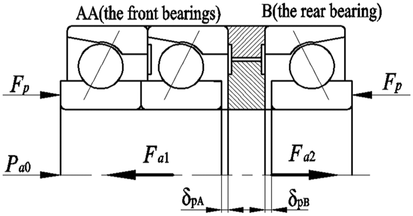
Combination bearings with preload and thrust load.

Bearing contact angular α_p and pre-deformation δ_p can be solved by the following equation¹⁶

\begin{matrix} \frac{F_{p}}{Z {D_{w}}^{2} K} = \sin α_{p} {(\frac{\cos α^{0}}{\cos α_{p}} - 1)}^{1.5} \\ δ_{p} = \frac{B D_{w} \sin (α_{p} - α^{0})}{\cos α_{p}} \end{matrix}

(1)

where

F_{p} = ζ \cdot ζ_{1} \cdot ζ_{2} \cdot ζ_{3} \cdot F_{A}

(2)

where F_A is the preload of the uninstalled bearings, and ζ is the bearing factor, ζ₁ is the correction factor of the bearing contact angle, ζ₂ is the correction factor of the preload grade, and ζ₃ is the correction factor of the bearing rolling element, and these parameters can be looked up in the bearing sample. Under the preload F_p, the front bearings generate axial displacement δ_pA, the rear bearing generates axial displacement δ_pB, and the total displacement is δ_p = δ_pA + δ_pB.

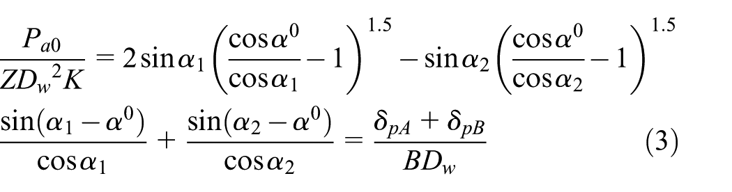
When the thrust force P_a₀ is applied on the preloaded combination bearings, entirety axial displacement δ_a₀ is generated. With the pre-deformation δ_p, the relationship between the contact angle of the front bearing α₁ and the rear bearing α₂ can be expressed as follows¹⁶

\begin{matrix} \frac{P_{a 0}}{Z {D_{w}}^{2} K} = 2 \sin α_{1} {(\frac{\cos α^{0}}{\cos α_{1}} - 1)}^{1.5} - \sin α_{2} {(\frac{\cos α^{0}}{\cos α_{2}} - 1)}^{1.5} \\ \frac{\sin (α_{1} - α^{0})}{\cos α_{1}} + \frac{\sin (α_{2} - α^{0})}{\cos α_{2}} = \frac{δ_{pA} + δ_{pB}}{B D_{w}} \end{matrix}

(3)

Frictional heat generation of the spindle-bearing system

Frictional heat generation of bearings is the dominant heat source in a spindle-bearing system, and it is mainly related to bearing internal speeds, dynamic loads, and lubrication state in the bearing. These factors will be discussed fully in the following sections.

Contact friction in the elastohydrodynamic lubrication of grease

Rolling bearings are generally operated with oil lubrication. Rolling element–raceway contact friction depends on contact geometry and load, rolling speed, and lubricant properties. A lubricant is a substance that is used to reduce friction and provide smooth running. Based on the Hertz elastic contact theory and Reynolds hydrodynamic lubrication theory, oil film thickness can be approximately calculated by considering the surface roughness.^17–25

For the contact of real surfaces, Weierstrass–Mandelbrot model can be used for the lubricated contact. An optical topographer is used to measure a profile in an arbitrary direction x²¹

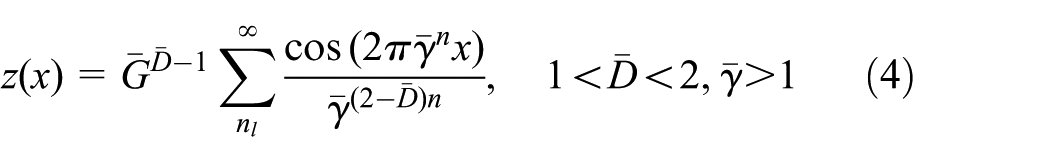
z (x) = {\bar{G}}^{\bar{D} - 1} \sum_{n_{l}}^{\infty} \frac{\cos (2 π {\bar{γ}}^{n} x)}{{\bar{γ}}^{(2 - \bar{D}) n}}, 1 < \bar{D} < 2, \bar{γ} > 1

(4)

where $\bar{D}$ is the fractal dimension, $\bar{G}$ is the characteristic scale coefficient, $\bar{γ}$ is an arbitrary parameter, and the value is usually 1.5. n_l is the minimum cutoff frequency of contour structure.

The mean square height, slope, and second derivative of a profile in an arbitrary direction are explained as follows¹⁹

m_{0} = E (z^{2}) = s^{2}, m_{2} = E [{(\frac{dz}{dx})}^{2}], m_{4} = E [{(\frac{d^{2} z}{d x^{2}})}^{2}]

(5)

where m₀, m₂, and m₄ are known as the zeroth, second, and fourth spectral moments of a profile, respectively.

The parameter Λ was established during the 1960s to indicate the degree to which a lubricant film separates the surfaces in rolling “contact”²⁰

Λ = \frac{h_{min}}{{(s_{m}^{2} + s_{R}^{2})}^{\frac{1}{2}}}

(6)

where s_m is the root mean square (rms) roughness of the raceway, and s_R is the rms roughness of the rolling element. Full-film separation can be assumed for Λ ≥ 3. When the lubricant film is insufficient to completely separate the surfaces in rolling contact, that is, for Λ ≤ 3, it is possible that some of the surface peaks, also called asperities, break through the lubricant film and contact each other when the lubricant temperature in the contact increases causing viscosity to decrease.

The ratio of contact to apparent area A_c/A₀ is¹⁹

\frac{A_{c}}{A_{0}} = π R_{s} S_{s} D_{SUM} F_{1} (\frac{d}{S_{s}})

(7)

where R_s is the assumed constant radius of the spherical summits, S_s is the standard deviation of the summit height distribution, D_SUM is the area density of summits, and d is the distance between the summit height and the surface mean plane. F₁(t) is the integral¹⁹

F_{1} (t) = \int_{t}^{\infty} (x - t) ϕ (x) dx

(8)

Other variables can be expressed as follows¹⁹

\begin{matrix} R_{s} = \frac{3}{8} {(\frac{π}{m_{4}})}^{\frac{1}{2}}, S_{s} = {[(1 - \frac{0.8968}{(m_{0} m_{4} / m_{2}^{2})}) m_{0}]}^{\frac{1}{2}} \\ D_{SUM} = \frac{m_{4}}{6 π m_{2} \sqrt{3}}, \frac{d}{S_{s}} = \frac{\frac{h}{m_{0}^{\frac{1}{2}}} - \frac{4}{{(π m_{0} m_{4} / m_{2}^{2})}^{\frac{1}{2}}}}{{(1 - \frac{0.8968}{(m_{0} m_{4} / m_{2}^{2})})}^{\frac{1}{2}}} \end{matrix}

(9)

Hamrock and Dowson proposed the calculation formula of dimensionless oil film thickness²⁶

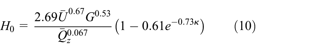
H_{0} = \frac{2.69 {\bar{U}}^{0.67} G^{0.53}}{{\bar{Q}}_{z}^{0.067}} (1 - 0.61 e^{- 0.73 κ})

(10)

where

G = λ E', \bar{U} = \frac{η_{0} U}{E' R_{x}}, {\bar{Q}}_{z} = \frac{Q}{E' R_{x}^{2}}, E' = \frac{E}{1 - ξ^{2}}

In the expression for H_o, the equivalent radius in the direction of rolling is given by

R_{x} = \frac{D_{w}}{2} (1 \mp γ)

(11)

The velocities U, with grease swept into the rolling element–raceway contacts, for the inner and outer raceway contacts are given by²⁶

\begin{matrix} U_{i} = \frac{d_{m}}{2} [(1 - γ) (ω - ω_{m}) + γ ω_{R}] \\ U_{o} = \frac{d_{m}}{2} [(1 + γ) ω_{m} + γ ω_{R}] \end{matrix}

(12)

Thickness of oil film center can be expressed as

h_{0} = H_{0} \cdot R_{x}

(13)

Point-contact oil film thickness in elastohydrodynamic lubrication (EHL) can be expressed as follows

h (x, y) = h_{0} + \frac{x^{2}}{2 R_{x}} + \frac{y^{2}}{2 R_{y}} + δ (x, y)

(14)

where h₀ is the oil film thickness of contact center; R_x and R_y are the equivalent curvature radii along the x, y direction; and δ(x, y) is the deformation displacement.

At high bearing operating speeds, some of the frictional heat generated in each concentrated contact is dissipated in the lubricant momentarily residing in the inlet zone of the contact. This effect tends to increase the temperature of the lubricant in the contact. It is clear that the lubricant dynamic viscosity will be changed as a result of temperature increase in the contact. Roelands established an equation which defined the relationship of dynamic viscosity, temperature, and pressure²⁶

\begin{array}{l} η (T, σ) = η_{0} \exp \\ {(\ln η_{0} + 9.67) [{(1 + 5.1 \times 10^{- 9} σ)}^{0.68} \times {(\frac{T - 138}{T_{0} - 138})}^{- 1.1} - 1]} \end{array}

(15)

Sliding motions and dynamic loads in ball bearings

Based on the Hertzian contact theory, the ball contacts the outer-ring and inner-ring raceways, such that the normal force Q is distributed over an elliptical surface defined by the projected major and minor axes 2a_n, 2b_n, respectively, as shown in Figure 3. The radius of a contact point (x_n, y_n) is defined as follows

r'_{n} = {{[{(R_{n}^{2} - x_{n}^{2})}^{\frac{1}{2}} - {(R_{n}^{2} - a_{n}^{2})}^{\frac{1}{2}} + {({(\frac{D_{w}}{2})}^{2} - a_{n}^{2})}^{\frac{1}{2}}]}^{2} + x_{n}^{2}}^{\frac{1}{2}}

(16)

Figure 3.

Model of ball and raceway contact.

Sliding of the raceway over the ball in the direction of rolling is determined by the difference between the linear velocities of raceway and ball. Hence, the sliding velocities in the y′ (rolling motion) and x′ (gyroscopic motion) directions are determined as follows²⁶

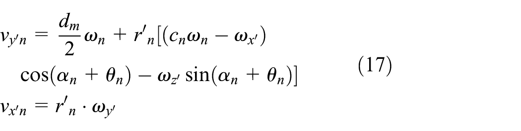
\begin{array}{l} v_{y^{'} n} = \frac{d_{m}}{2} ω_{n} + {r^{'}}_{n} [(c_{n} ω_{n} - ω_{x^{'}}) \cos (α_{n} + θ_{n}) - ω_{z^{'}} \sin (α_{n} + θ_{n})] \\ v_{x^{'} n} = {r^{'}}_{n} \cdot ω_{y^{'}} \end{array}

(17)

where

θ_{n} = arc \sin (\frac{x_{n}}{r_{n}})

In equation (16), c_o = 1 and c_i = −1. The friction shear stress is described as given by Harries and Barnsby

τ = c_{v} \frac{A_{c}}{A_{0}} μ_{a} σ + (1 - \frac{A_{c}}{A_{0}}) {[{(η \frac{v}{h})}^{- 1} + τ_{lim}^{- 1}]}^{- 1}

(18)

where A_c is the area associated with the asperity–asperity contact, A₀ is the total contact area, and sliding coefficient c_v = 1 or −1 depending on the direction of sliding velocity.

As shown in Figure 4, the relative axial displacement of the inner rings is δ_a, and the relative angular displacements is θ; the axial distance between the loci of inner and outer raceway curvature centers at the ball position is A₁. In accordance with a relative radial displacement of the ring centers δ_r, the radial displacement between the loci of the curvature centers at each ball position is A₂; changes of the two positions can be expressed as follows²⁶

\begin{matrix} A_{1} = B D_{w} \sin α^{0} + δ_{a} \\ A_{2} = B D_{w} \cos α^{0} + δ_{r} \end{matrix}

(19)

Figure 4.

Position of the ball center and raceway groove curvature center.

The position variables X₁, X₂, A₁, A₂ are related to contact angles α_i and α_o and contact deformations δ_i and δ_o as follows

\begin{matrix} \cos α_{o} = \frac{X_{2}}{(f_{o} - 0.5) D_{w} + δ_{o}}, \sin α_{o} = \frac{X_{1}}{(f_{o} - 0.5) D_{w} + δ_{o}} \\ \cos α_{i} = \frac{A_{2} - X_{2}}{(f_{o} - 0.5) D_{w} + δ_{i}}, \sin α_{i} = \frac{A_{1} - X_{1}}{(f_{o} - 0.5) D_{w} + δ_{i}} \end{matrix}

(20)

The remaining two equations pertaining to the position of the ball center can be obtained

\begin{matrix} {(A_{1} - X_{1})}^{2} + {(A_{2} - X_{2})}^{2} - {[(f_{i} - 0.5) D_{w} + δ_{i}]}^{2} = 0 \\ X_{1}^{2} + X_{2}^{2} - {[(f_{o} - 0.5) D_{w} + δ_{o}]}^{2} = 0 \end{matrix}

(21)

Friction shear stresses can be calculated by a given lubricating fluid and a given condition of rolling contact surface separation.²⁷Figure 5 shows the force and moment loads of a ball in loaded, grease-lubricated angular-contact ball bearing.

Figure 5.

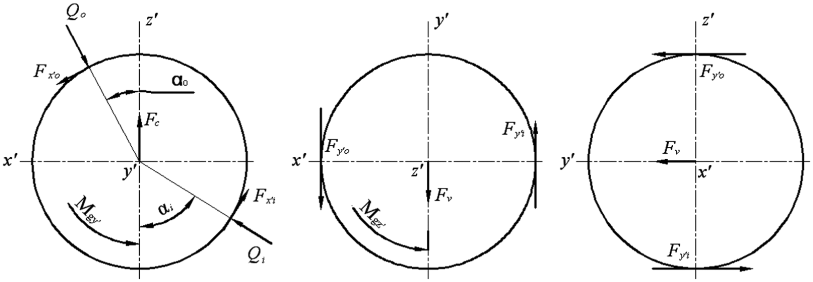
Ball model with forces and moments.

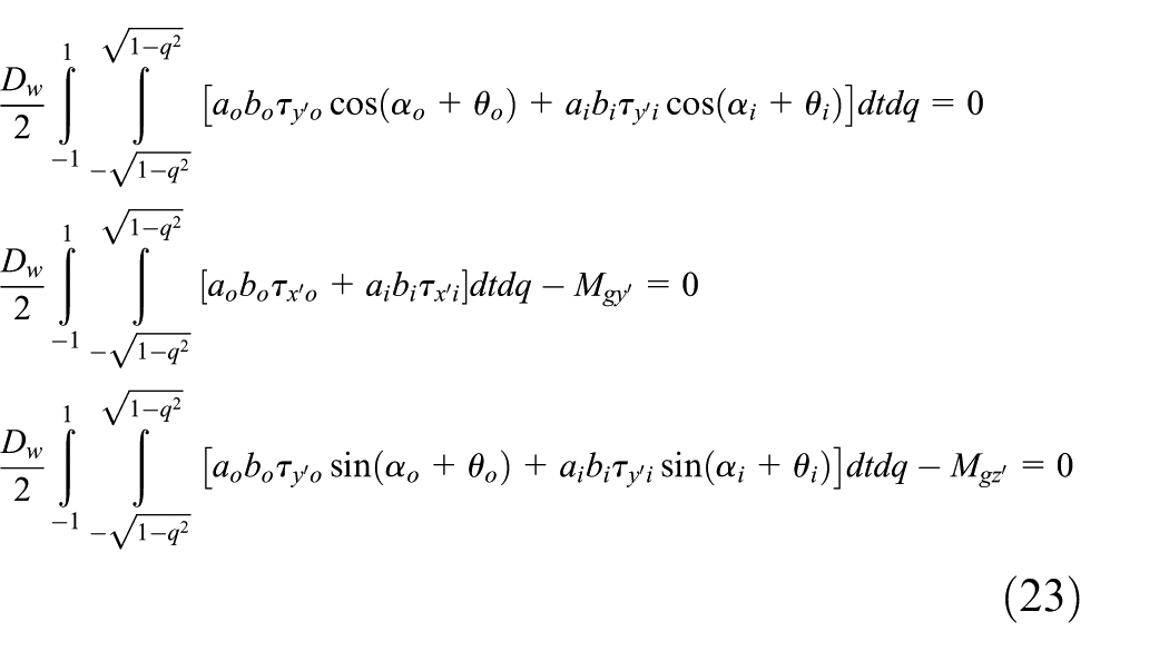
From Figure 5, it can be seen that the following conditions of force equilibrium must be satisfied for steady-state operation of the bearing²⁶

\begin{matrix} Q_{o} \cos α_{o} - Q_{i} \cos α_{i} - F_{x' o} \sin α_{o} + F_{x' i} \sin α_{i} - F_{z'} = 0 \\ Q_{o} \sin α_{o} - Q_{i} \sin α_{i} + F_{x' o} \cos α_{o} - F_{x' i} \cos α_{i} = 0 \\ F_{y' o} - F_{y' i} + F_{v} = 0 \\ Q_{o} \sin α_{o} + F_{x' o} \cos α_{o} - F_{a} / Z = 0 \end{matrix}

(22)

Viscous drag force F_v in equation (22) can be expressed as

F_{v} = \frac{μ_{v} π ρ D_{w}^{2} {(d_{m} ω_{m})}^{1.95}}{32 g}

where ρ is the weight of the lubricant in the bearing free space divided by the volume of the free space, and µ_v is the drag coefficient.

The moment equilibrium conditions are

\begin{matrix} \frac{D_{w}}{2} \int_{- 1}^{1} \int_{- \sqrt{1 - q^{2}}}^{\sqrt{1 - q^{2}}} [a_{o} b_{o} τ_{y' o} \cos (α_{o} + θ_{o}) + a_{i} b_{i} τ_{y' i} \cos (α_{i} + θ_{i})] dtdq = 0 \\ \frac{D_{w}}{2} \int_{- 1}^{1} \int_{- \sqrt{1 - q^{2}}}^{\sqrt{1 - q^{2}}} [a_{o} b_{o} τ_{x' o} + a_{i} b_{i} τ_{x' i}] dtdq - M_{gy'} = 0 \\ \frac{D_{w}}{2} \int_{- 1}^{1} \int_{- \sqrt{1 - q^{2}}}^{\sqrt{1 - q^{2}}} [a_{o} b_{o} τ_{y' o} \sin (α_{o} + θ_{o}) + a_{i} b_{i} τ_{y' i} \sin (α_{i} + θ_{i})] dtdq - M_{gz'} = 0 \end{matrix}

(23)

According to static analysis results, variables in equations (22) and (23) are given initial values; the unknown variables have been solved by the iterative method.

Friction heat generation

In the ball–raceway contact, rate of the friction heat generation is given by²⁶

\begin{matrix} {\overset{\cdot}{E}}_{nyj} = \frac{1}{J} \int τ_{nyj} υ_{nyj} d A_{nj} = \frac{a_{nj} b_{nj}}{J} \\ \int_{- 1}^{1} \int_{- \sqrt{1 - q^{2}}}^{\sqrt{1 - q^{2}}} τ_{nyj} υ_{nyj} dtdq n = i, o; j = 1, 2, \dots, Z \\ {\overset{\cdot}{E}}_{nxj} = \frac{1}{J} \int τ_{nxj} υ_{nxj} d A_{nj} = \frac{a_{nj} b_{nj}}{J} \\ \int_{- 1}^{1} \int_{- \sqrt{1 - q^{2}}}^{\sqrt{1 - q^{2}}} τ_{nxj} υ_{nxj} dtdq n = i, o; j = 1, 2, \dots, Z \end{matrix}

(24)

where J is a constant converting to W; the surface friction shear stress and the sliding velocity are obtained from the above section.

For a grease-lubricated bearing, in addition to the friction heat generated in the ball–raceway contacts, friction heat is also generated due to the balls passing through the lubricant and is given by

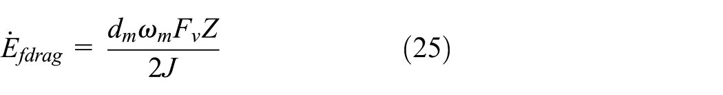
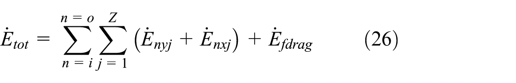
{\overset{\cdot}{E}}_{fdrag} = \frac{d_{m} ω_{m} F_{v} Z}{2 J}

(25)

Rate of the total friction heat generation is obtained by summation of the component heat generations

{\overset{\cdot}{E}}_{tot} = \sum_{n = i}^{n = o} \sum_{j = 1}^{Z} ({\overset{\cdot}{E}}_{nyj} + {\overset{\cdot}{E}}_{nxj}) + {\overset{\cdot}{E}}_{fdrag}

(26)

Heat transfer model and temperature distribution

Three fundamental modes for the transfer of the friction heat among the shaft, bearings, and housing are the heat conduction, heat convection, and heat radiation. Heat radiation effect is minor and usually be neglected.

The heat conduction includes the inner-ring shaft, outer-ring housing, and inner and outer raceway balls. The heat convection includes the grease lubrication, oil cooling, and ambient air.¹¹Figure 6 shows the thermal resistances and temperature nodes model along the radial direction of the front bearing. Nine axial temperature nodes and eight radial temperature nodes are defined. All temperature nodes and corresponding heat transfer equations are calculated by Takabi and Khonsari.²⁸

Figure 6.

Temperature and thermal resistance model along the radial direction of the spindle system.

Burton and Steph³⁰ proposed that half of the friction heat is transferred to balls, and the other half is transferred to the rings. It can be calculated by standard finite difference methods. The spindle is decomposed into a certain amount of nodes for analyzing. At each node, heat influx equals heat efflux; therefore, the sum of all heat flowing toward a temperature node is equal to zero, as shown in Figure 7.

Figure 7.

Two-dimensional temperature node system.

From the figure, the heat flows in a node can be expressed as

{\overset{\cdot}{E}}_{f 0} + {\overset{\cdot}{E}}_{1 - 0, c} + {\overset{\cdot}{E}}_{2 - 0, v} + {\overset{\cdot}{E}}_{3 - 0, c} + {\overset{\cdot}{E}}_{4 - 0, c} = 0

(27)

where ${\overset{\cdot}{E}}_{f 0}$ is the heat generation; ${\overset{\cdot}{E}}_{1 - 0, c}$ , ${\dot{E}}_{2 - 0, v}$ , ${\overset{\cdot}{E}}_{3 - 0, c}$ , ${\overset{\cdot}{E}}_{4 - 0, c}$ are the heat flows by the heat conduction; and ${\overset{\cdot}{E}}_{2 - 0, v}$ is the heat flow by the convection. Based on Newton’s law of cooling and Fourier’s law, equation (27) can be expressed as

{\dot{E}}_{f o} + \frac{1}{R_{1}} \cdot (T_{1} - T_{0}) + Π_{2} \cdot S_{2} \cdot (T_{2} - T_{0}) + \frac{1}{R_{3}} \cdot (T_{3} - T_{0}) + \frac{1}{R_{4}} \cdot (T_{4} - T_{0}) = 0

(28)

For all nodes of the spindle system, thermal contact resistance and heat transfer coefficients can be obtained from previous works.^27–30 Conductive and convective resistance formulas for the spindle-bearing system presented in Table 1 with the corresponding Re and Pr also are presented in this table. Equations similar to equation (28) can be written and solved by the Newton–Raphson method.

Table 1.

Conductive and convective resistance formulas for the spindle-bearing system.

Thermal resistance	Conductive and convective resistance formulas
$R_{ob}, R_{ib}$	$R = \frac{ψ (a / b)}{4 ka}, ψ (a / b) = \frac{2}{π} \int_{0}^{π / 2} \frac{d θ}{\sqrt{[1 - {(1 - b^{2} / a^{2})}^{2} \sin^{2} θ]}}$
$R_{b}$	$R = \frac{2}{π k D_{w}}$
$R_{l}$	$1 / (Π_{l} \cdot S) = 1 / (0.332 k \Pr^{\frac{1}{3}} \cdot {(\frac{u_{m}}{ν x})}^{\frac{1}{2}} \cdot S)$
$R_{f}$	$\begin{matrix} 1 / (Π_{f} \cdot S) = 1 / (0.0225 \cdot \frac{k}{h_{gap}} \cdot {Re}^{0.8} \cdot \Pr^{0.3} \cdot S) \\ or 1 / (Π_{f} \cdot S) = 1 / (1.86 \cdot \frac{k}{h_{gap}} \cdot {(Re \cdot \Pr \cdot \frac{h_{gap}}{L})}^{\frac{1}{3}} \cdot S) \\ where Re = \frac{u \cdot h_{gap}}{ν}, P_{r} = \frac{c \cdot η}{k} \end{matrix}$
$R_{h}, R_{o}, R_{i}, R_{s}$	$R = \frac{1}{k} \frac{\ln (D_{o} / D_{i})}{2 π b}$
$R_{lb}$	$1 / (Π_{v} \cdot S) = 1 / (0.33 \frac{κ}{D} {Re}_{D}^{0.5} \Pr^{0.4} \cdot S)$
$R_{oh}$	$R = (\frac{h_{ring}}{k_{ring}} + \frac{h_{gap}}{k_{gap}}) / S$
$R_{air}$	$R = 1 / ((c_{0} + c_{1} \cdot u^{c_{2}}) \cdot S)$

Experimental setup and data reduction

Experimental setup

The experimental apparatus is shown in Figure 8. The spindle system is tested by five sets of Micro-Epsilon laser triangulation sensors measurement instrument and FLIR’s thermal infrared imager. The spindle is operated in an air-conditioned environment, and the temperature is 17.6°C. The spindle is cooled by Habor Oil Cooler, the model is HBO-3RPTSB-BY-10, and the oil temperature can be controlled between 10°C and 40°C. In the experiment, the initial temperature of cooling oil is 15°C. There are five temperature measurement points SP01–SP05: SP01–SP03 measured the front bearings, SP04 measured the middle part between the front bearing and the rear bearing, and SP05 measured the rear bearing. All data signals were collected and converted by data acquisition system. Figure 9 shows the measured temperature curve. The test is continued until the steady-state condition is attained. Minimum of 3.5 h was required for the temperature measurements to become steady. Test is stopped upon attainment of the steady state by shutting down the spindle motor. When the spindle is reaching the thermal balance, the temperature is changed very small; we consider this steady state as the thermal balance. It means that the rate of heat generation inside and the rate of heat dissipation from the bearing reach a state of equilibrium. The time to reach thermal balance is different for each combination of rotational speed and load, but we did hundreds of tests, the longest time was almost 4 h except of thermal failure which happened before it reached the steady state.

Figure 8.

Measurement system of the spindle.

Figure 9.

Measured temperature for test condition of 3000 r/min and 1750 N thrust load.

Data reduction

The experimental spindle of the horizontal machining center is operated at eight different speeds from 0 to 4500 r/min, and the interval is 500 r/min. When the measured points have small temperature changes at the minimum speed, the speed adjusts to the next value, until reaching the maximum speed. Acquisition and pickup temperature data and the experimental temperatures are shown in Figure 10.

Figure 10.

Measured temperature during step test from 0 to 4500 r/min.

Results and discussions

In order to verify validity of numerical analysis models presented in sections “Frictional heat generation of the spindle-bearing system” and “Experimental setup and data reduction,” different spindle running conditions are set, experiments and simulations can be compared under operating conditions. Then the mathematical model provides theory analysis for optimum design and dynamic compensation of machine tool spindle system.

Numerical results

In this article, Kluber/NBU 15 grease is used to lubricate the spindle bearing. It has a kinematic viscosity of 21 mm²/s at 40°C and 4.7 mm²/s at 100°C, and the density of grease is 0.99 g/cm³. The dynamic viscosity–temperature curve is shown in Figure 11.

Figure 11.

Viscosity of lubricating grease versus temperature.

Wilson developed thermal reduction factors for lubricant film thickness from numerical solutions of the thermal EHL problem for rolling–sliding contacts. The film thickness reduction factor is taken into account,²⁶ the oil film thickness of contact center in the front bearings can be calculated, and the result is shown in Figure 12.

Figure 12.

Oil film thickness of the grease in contact center.

Figure 12 shows comparison of central oil film thickness in the isothermal state and thermal effect on the grease. As seen, in the isothermal state, center oil film would be thicker at higher rotational speed. Since when the grease temperature is increasing, grease viscosity will decrease. Center oil film thickness will increase more slowly with considering thermal effect, especially at high speed, oil film thickness even decrease, and then the friction shear stress will be changed greatly, leading to an non-ignorable effect on friction heat generation.

In this article, the spindle bearing (71928CD/P4ATBTA) is a triple angular-contact ball bearing; the suffix TBT represents tandem duplex and back-to-back combination mode. Corresponding to 1.1 million DN with a 165 mm bore diameter of the spindle bearings, the ball diameter is 13.37 mm. The supporting bearing (71924CD/P4ADBA) is a back-to-back combination bearing; the suffix DB represents back-to-back combination mode. The spindle system was operated under 1137.2 N preload, which is provided by the adjustable ring. Variables of ball–raceway contacts under different speeds are calculated using non-isothermal lubricant, and the calculated results are shown in Figures 13 –15. From the figures, it is clear that axial load, centrifugal forces, gyroscopic moments, and lubrication conditions can significantly influence bearing contact deflections, contact angles, and contact loads.

Figure 13.

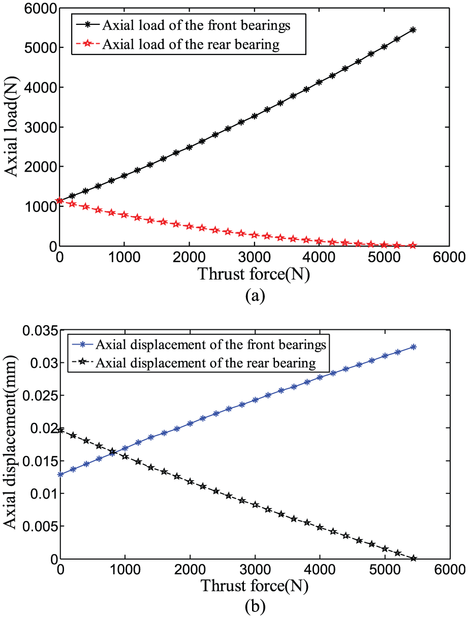
Axial load and axial displacement versus thrust force: (a) axial load calculated based on the constant preload of 1137.2 N and (b) axial displacement calculated based on the constant preload of 1137.2 N.

Figure 14.

Calculated variables of rolling elements in the spindle bearings: (a) ball–inner raceway and ball–outer raceway normal contact deformations δ_ij and δ_oj, (b) ball–inner raceway and ball–outer raceway normal contact angles α_ij and α_oj, and (c) semi-major and semi-minor axes of the elliptic contact in inner and outer raceway.

Figure 15.

Ball speeds of the spindle bearings.

According to equation (6) and the experimental results of rough surface, the simulation results of parameter Λ at the 0° position are shown in Figure 16. Area associated with the asperity–asperity contact can be negligible, the friction shear stress is governed by the grease in the contact, and the friction heat generations of the spindle bearings are calculated by equations (24) and (25). The calculated results are obtained as shown in Figure 17. All temperature nodes and corresponding heat transfer equations are calculated, and the calculated results are shown in Figure 18. From Figure 18, it can be seen that temperature gradient is high, and rate of the heat dissipation from the bearing outer ring is higher than that from the inner ring.

Figure 16.

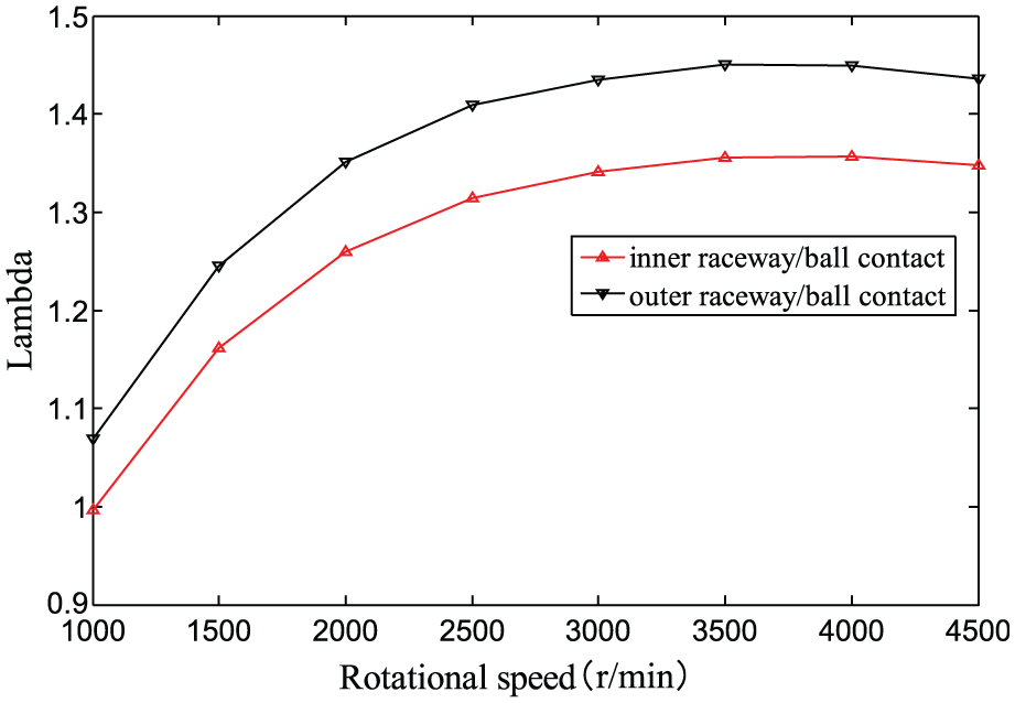
Lambda parameters at the 0° position of the spindle bearing.

Figure 17.

Frictional heat generation.

Figure 18.

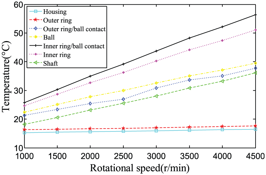
Temperature distribution of spindle.

Comparison with experimental results

Acquisition and pickup temperature data are compared with the corresponding simulation data. The experimental temperatures and numerical ones are shown in Figure 19. From the figure, the temperature predictions for 2000 and 2500 r/min are less accurate; this is mainly due to the difficulty in predicting thermally induced preload and lubrication condition in these speeds. But, on the whole, prediction temperatures are in good agreement with the experimental results. Therefore, it can be said that the numerical model can be applied to analyze the thermal characteristics and improve spindle design.

Figure 19.

Comparison of temperatures.

Optimization and analysis of the cooling system

From Figure 18, it can be seen that a large temperature difference occurs, and the thermal balance is not stable. If the spindle works for a long time, the instability increases the ball–raceway contact load, friction, and temperature, which results in the bearing seizure. So the cooling system is used to balance the temperature gradient of the spindle system.

For the oil-cooling system, physical model of the spindle system with a helical rectangular oil-cooling channel is shown in Figure 20. The convective heat transfer of cooling oil changes with the flow type. Type of the flow around the housing surface is divided into turbulent and laminar.

Figure 20.

Physical model of cooling system with the cylindrical channel.

The cooling oil used is ISO VG32; its physical properties are functions of temperature, from physical parameters of the cooling oil, and the equations are obtained by the curve-fitting method as

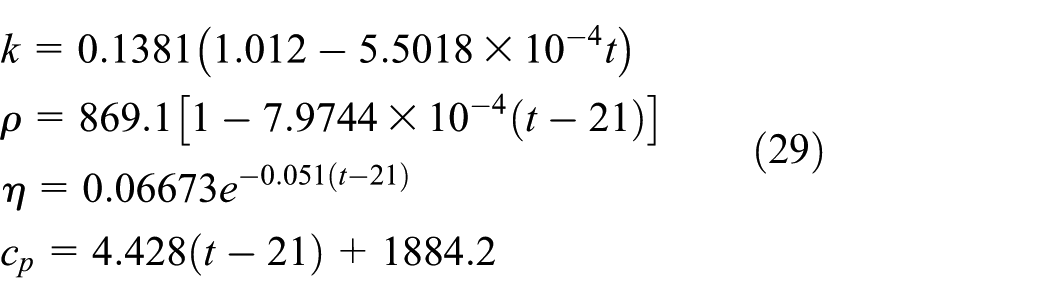
\begin{matrix} k = 0.1381 (1.012 - 5.5018 \times 10^{- 4} t) \\ ρ = 869.1 [1 - 7.9744 \times 10^{- 4} (t - 21)] \\ η = 0.06673 e^{- 0.051 (t - 21)} \\ c_{p} = 4.428 (t - 21) + 1884.2 \end{matrix}

(29)

As shown in Figure 21, the simulation results and the experimental measurements are in good agreement in both trend and magnitude. So the simulation results can be used to calculate the convective heat transfer coefficients of the fluid.

Figure 21.

Physical characteristics of cooling fluid: (a) heat conductivity coefficient, (b) density, (c) dynamic viscosity, and (d) specific heat capacity.

According to the Nusselt criterion, when the cooling oil is under the condition of turbulent flow state, the convective heat transfer coefficient can be calculated as follows

Π_{f} = 0.0225 \cdot u^{0.8} \cdot h_{gap}^{- 0.2} (k^{0.7} \cdot ρ^{0.8} \cdot c^{0.3} \cdot η^{- 0.5})

(30)

Under the condition of laminar flow state, the convective heat transfer coefficient can be calculated according to the following formula

Π_{f} = 1.86 \cdot u^{\frac{1}{3}} \cdot {(h_{gap} \cdot L)}^{- \frac{1}{3}} {(k^{2} \cdot ρ \cdot c)}^{\frac{1}{3}}

(31)

From equations (30) and (31), it can be seen that the temperature of the cooling oil and sectional dimensions of the cooling channel are the important variables for calculating coefficient of convection heat transfer. The heat transfer coefficient equation of the cooling oil is transformed to a function with temperature and h_gap variables. According to the structure finite element analysis, value range of h_gap is from 0.005 to 0.03 m, the step is 0.005 m; value range of oil temperature is from 10°C to 40°C. Relationship between the heat transfer coefficients, temperature, and gap characteristic dimension h_gap is shown in Figure 22.

Figure 22.

Coefficients versus temperatures of cooling fluid.

When gap characteristic dimension h_gap is less than 0.01 m, the temperature has a minimal effect on the convection heat transfer coefficient of the cooling fluid, and the fluid is obvious in laminar flow. When h_gap is greater than 0.01 m, the state of the cooling fluid changes from laminar flow to turbulent flow with the increase in temperature, and the broken line is the turning point of the fluid state. In the turbulent state, the convection heat transfer increases very quickly when the temperature increases.

Based on cooling channel machining condition, and the cooing capability of oil cooler, according to the calculated results of equations (30) and (31), the optimal value of coefficient of convective heat transfer can be obtained after restudy of the physical parameters, and the optical physical parameters of cooling channel and oil cooler also can be obtained; optimal value h_gap is 19 mm, and the optimal temperature is 31°C.Figure 22 is obtained with cooling oil of 31°C and h_gap of 19 mm. Figure 23 shows that the maximum temperature is higher than that in Figure 18, but the increasing value is less than 3°C, and it has little effect on temperature distribution of the spindle system. The temperature difference across the bearing is lesser than that in Figure 18, and the decreasing value is about 15°C. This optimized cooling system can maintain the temperature gradient across the bearing.

Figure 23.

Temperature along the radial direction after optimization.

In this article, a computer program is developed to implement analysis and calculation for a given spindle configuration and operational conditions, the thermal information and optimized parameters can be obtained, and this is useful to provide dynamic compensation for working machining center and improve the machining center structure in the R&D.

Conclusion

An analysis and modeling procedure for simulating friction heat generation of the spindle system has been developed. Thrust force, rotational speed, lubrication condition, and surface asperities are calculated in detail. The model provides a practical model for the thermal characteristics of the spindle-bearing system due to the finite number of thermal nodes in the heat transfer model of the spindle system in the radial direction.

The heat transfer capability of the cooling system is related to the cooling oil temperature, the cooling oil flow, and the equivalent diameter of the cooling channel. The cooling oil flow is selected the maximum flow, and then the relationship of the heat transfer coefficient of the cooling system, the cooling oil temperature, and the equivalent diameter of the cooling channel is analyzed.

The system temperature gradient is mainly determined by the cooling system, as well as the applied force and speed. Cooling channel sectional dimensions and cooling oil temperature are the main parameters to optimize temperature gradient of the spindle system.

Footnotes

Appendix 1

Academic Editor: Ramoshweu Lebelo

Declaration of conflicting interests

The author(s) declared no potential conflicts of interest with respect to the research, authorship, and/or publication of this article.

Funding

The author(s) received no financial support for the research, authorship, and/or publication of this article.

References

Min

Shuyun

Ying

An improved thermal model for machine tool bearings. Int J Mach Tool Manu 2007; 47: 53–62.

Lin

C-W

Kamman

An integrated thermo-mechanical-dynamic model to characterize motorized machine tool spindles during very high speed rotation. Int J Mach Tool Manu 2003; 43: 1035–1050.

Choi

Lee

DG.

Thermal characteristics of the spindle bearing system with a gear located on the bearing span. Int J Mach Tool Manu 1998; 38: 1017–1030.

Twardowski

Legutko

Krolczyk

. Investigation of wear and tool life of coated carbide and cubic boron nitride cutting tools in high speed milling. Adv Mech Eng 2015; 7: 1–9

Stein

JF.

A state-space model for monitoring thermally induced preload in anti-friction spindle bearings of high-speed machine tools. J Dyn Syst: T ASME 1994; 116: 372–386.

Stein

JL.

On-line preload monitoring for anti-friction spindle bearings of high-speed machine tools. J Dyn Syst: T ASME 1995; 117: 43–53.

Stein

JL.

Active thermal preload regulation for machine tool spindles with rolling element bearings. J Manuf Sci E: T ASME 1996; 118: 499–505.

JF.

Thermoelastic instability monitoring for preventing spindle bearing seizure. Tribol T 1995; 38: 11–18.

Katter

JG.

Bearing force monitoring in a three-shift production environment. Tribol T 1996; 39: 201–207.

10.

Katter

JF.

Bearing condition monitoring for preventive maintenance in a production environment. Tribol T 1996; 39: 936–942.

11.

Bossmanns

JF.

A thermal model for high speed motorized spindles. Int J Mach Tool Manu 1999; 39: 1345–1366.

12.

Bossmanns

JF.

A power flow model for high speed motorized spindles—heat generation characterization. J Manuf Sci E: T ASME 2001; 123: 494–505.

13.

Holkup

Cao

Kolář

. Thermo-mechanical model of spindles. CIRP Ann: Manuf Techn 2010; 59: 365–368.

14.

Mizuta

Inoue

Takahashi

. Heat transfer characteristics between inner and outer rings of an angular ball bearing. Heat Transf: Asian Res 2003; 32: 42–57.

15.

Chien

Jang

JY.

3-D numerical and experimental analysis of a built-in motorized high-speed spindle with helical water cooling channel. Appl Therm Eng 2008; 28: 2327–2336.

16.

Harris

Kotzalas

MN.

Essential concepts of bearing technology: rolling bearing analysis. 5th ed.Boca Raton, FL: CRC Press, 2006.

17.

Hamrock

Dowson

Ball bearing lubrication: elastohydrodynamics of elliptical contact. New York: Wiley, 1981, pp.1–386.

18.

Jang

Cho

Barber

JR.

The thermoelastic Hertzian contact problem. Int J Solids Struct 2009; 46: 4073–4078.

19.

McCool

JI.

Comparison of models for the contact of rough surfaces. Wear 1986; 107: 37–60.

20.

Dowson

Elastohydrodynamic and micro-elastohydrodynamic lubrication. Wear 1995; 190: 125–138.

21.

Greewood

JJ.

Surface roughness and contact: an apology. Meccanica 2001; 36: 17–630.

22.

Masjedi

Khonsari

MM.

Theoretical and experimental investigation of traction coefficient in line-contact EHL of rough surfaces. Tribol Int 2014; 70: 79–189.

23.

Takabi

Khonsari

MM.

On the dynamic performance of roller bearings operating under low rotational speeds with consideration of surface roughness. Tribol Int 2015; 86: 2–71.

24.

Lugt

PM.

Grease lubrication in rolling bearings. New York: John Wiley & Sons, 2013.

25.

Lugt

PM.

A Review on grease lubrication in rolling bearings. Tribol T 2009; 52: 70–480.

26.

Harris

Kotzalas

MN.

Advanced concepts of bearing technology: rolling bearing analysis. 5th ed.Boca Raton, FL: CRC Press, 2006.

27.

Katsuhiko

Thermal contact resistance between balls and rings of a bearing under axial, radial, and combined loads. J Thermophys Heat Tr 1995; 9: 88–95.

28.

Takabi

Khonsari

MM.

Experimental testing and thermal analysis of ball bearings. Tribol Int 2013; 60: 3–103.

29.

Rohsenow

Hartnett

Cho

. Handbook of heat transfer. New York: McGraw-Hill, 1998.

30.

Burton

Staph

HE.

Thermally activated seizure of angular contact bearings. ASLE Trans 1967; 10: 408–417.

A study of cooling system in a grease-lubricated precision spindle

Abstract

Keywords

Introduction

Structure model of the spindle system

Frictional heat generation of the spindle-bearing system

Contact friction in the elastohydrodynamic lubrication of grease

Sliding motions and dynamic loads in ball bearings

Friction heat generation

Heat transfer model and temperature distribution

Experimental setup and data reduction

Experimental setup

Data reduction

Results and discussions

Numerical results

Comparison with experimental results

Optimization and analysis of the cooling system

Conclusion

Footnotes

Appendix 1

Declaration of conflicting interests

Funding

References