Theoretical analysis and finite element method simulations on dynamic sensitivity of hemisphere-shaped electrostatic sensors

Abstract

Electrostatic sensors are key components of electrostatic monitoring systems. Their sensitivity characteristics have a direct influence on monitoring accuracy. In previous studies, spatial sensitivity, which is called static sensitivity here, was used to describe the sensitivity characteristics. However, it only reflects a basic relationship between static charged particles and induced charges on an electrostatic sensor’s probe. Besides, as a three-dimensional defined parameter, it is difficult to build a unified model if actual boundary conditions are considered. Thus, it is not quite proper for applications that detect moving particles. To solve this problem, dynamic sensitivity is proposed in this article. As for a hemisphere-shaped electrostatic sensor, first, a more accurate model of static sensitivity is built. Based on it, dynamic sensitivity is defined and modeled analytically. Then, a calibration method is proposed to improve the model’s accuracy under actual boundary conditions. In the end, finite element method simulations are done for validations. The results demonstrate that dynamic sensitivity reflects a relationship between moving charged particles and the actual output signals of a sensor, thus it is direct and practical for moving particles. And the theoretical results are highly consistent with the simulated ones. Moreover, the dynamic sensitivity indicates localized sensing characteristics of hemisphere-shaped electrostatic sensors.

Introduction

Due to the advantages of robustness and low cost,^1–3 electrostatic monitoring has been widely used for parameter monitoring of gas–solid two-phase flows, such as flow velocity, mass flow rate, and flow pattern,^1–10 and detecting abnormal debris present in gas turbines’ exhaust gas for online condition monitoring.^11–16

Electrostatic sensors are key components in electrostatic monitoring systems. They are mainly divided into two types: intrusive and nonintrusive. ¹⁷ Typical intrusive ones are rod-shaped electrostatic sensors, which are often used for emission monitoring of gas turbines.^11–16 Fisher ¹⁶ researched an electrostatic monitoring system that consists of the ingested debris monitoring system (IDMS) and exhaust debris monitoring system (EDMS), where rod-shaped electrostatic sensors were used. Similarly, Zuo and coworkers^11,13,15 also applied rod-shaped electrostatic sensors to obtain condition signals from exhaust gas of aero-engines. Besides, Yan and coworkers^7,18 studied a kind of net installed intrusive electrostatic sensor, which was used for online monitoring of particle size. In general, intrusive sensors have advantages of relatively high sensitivity, easy installation, and flexible layout. However, they would interfere with the flow, which is not allowed in some dense two-phase flows in order to prevent obstruction and probe abrasion. In addition, it is difficult to study their sensitivity characteristics theoretically due to their shapes. Therefore, sensitivity characteristics of intrusive ones are usually studied using numerical methods based on finite element method (FEM) or experiments,^1,10 and accurate analytical models remain to be built. In order to overcome the drawbacks of intrusive sensors, nonintrusive ones have been studied, such as plate-shaped and ring-shaped electrostatic sensors.^2,4,6,8 Rahmat and coworkers^2,8 compared different-sized circular plate–shaped and rectangular plate–shaped electrostatic sensors and built their analytical models of spatial sensitivity. However, the models might be less accurate when influences of the pipeline shape are taken into consideration. In addition, a plate-shaped electrostatic sensor has relatively low sensitivity irrespective of the expansion of the plate’s dimensions. This would increase difficulties in manufacturing and installation. Xu et al.^3,4 studied the sensing characteristics and signal processing methods of ring-shaped electrostatic sensors, which were used for flow parameter monitoring.^1,19,20 However, a ring-shaped one only provides the integrated signals from all the particles present in the sensing zone, thus lacking local information for some monitoring objectives, such as flow pattern and fault location. By making a trade-off between the two types of electrostatic sensors, we proposed hemisphere-shaped electrostatic sensors. ¹⁷ They combine the advantages of intrusive electrostatic sensors and the nonintrusive ones. Moreover, since the probe size is much smaller than the radius of a pipeline, hemisphere-shaped electrostatic sensors cause very little disturbance to the flow. These advantages make them much promising in some popular applications, such as electrostatic tomography systems.^17,21–25 In general, electrostatic sensors are studied in macro-scale; thus, we just consider electrostatic induction as their basic physics. However, if being studied in nano-scale, the influence of dispersion forces,^26,27 surface effect, and size-effect^28–30 might be considerable in the behavior of electrostatic sensors, which is no longer discussed here. By making a commonly used simplification of the pipeline shape, an analytical model of hemisphere-shaped electrostatic sensors’ spatial sensitivity was built by us. ¹⁷ However, an implied condition in some latter integrate steps was not considered, which would affect the accuracy of the model to some extent. Beyond this, there have not been further papers on hemisphere-shaped electrostatic sensors yet.

Sensitivity characteristics, which are important to electrostatic sensors, have a direct influence on monitoring accuracy. ³ In previous studies,^3,11,31,32 spatial sensitivity was used to describe the sensitivity characteristics. It is defined as the absolute value of induced charges on an electrostatic sensor’s probe from a static unit point charge, thus we call it static sensitivity in the following. However, first, a charged particle is always moving in most applications; thus, the induced charges are changing continuously instead of static in fact. Besides, the change rate varies with the particles’ velocity which is difficult to obtain with a single electrostatic sensor. Second, the output signals of an electrostatic sensor are transformed into voltage signals for post-processing, instead of the original induced charges. Third, for the reason that static sensitivity is defined in the three-dimensional space, it is difficult to build a unified analytical model if the pipeline shape is taken into consideration; however, generally, not all the signals from the whole space are important in practice. As a result, it is hard to describe practical sensing characteristics of an electrostatic sensor by relationship between the static charged particles and the induced charges in the whole three-dimensional space. In another word, the generally used static sensitivity is not direct and practical for applications that detect moving charged particles, thus a new and more proper parameter is needed for this case. Besides, just as mentioned before, the type of an electrostatic sensor has much to do with building accurate analytical models of its sensitivity parameters.

In order to overcome the drawbacks of static sensitivity, dynamic sensitivity is proposed in this article. The term of dynamic sensitivity had been used once by Zhou et al., ³³ but its definition was quite different. In this article, dynamic sensitivity describes a relationship between moving charged particles and the actual output voltage signals, making it direct and practical for most applications. Moreover, as a two-dimensional defined parameter, it is easier to build a unified analytical model for dynamic sensitivity. As for a hemisphere-shaped electrostatic sensor, first, a more accurate analytical model of its static sensitivity is built by making an improvement from our previous work. ¹⁷ Based on it, the dynamic sensitivity is defined and modeled theoretically under a commonly used simplified boundary condition. Then, considering the effects of the pipeline shape, a calibration method is proposed to improve the model of dynamic sensitivity under actual boundary conditions. In the end, all of the theoretical results are validated using FEM simulations. In a word, this article provides improved models to describe the sensitivity characteristics of hemisphere-shaped electrostatic sensors and provides a more practical sensitivity parameter for electrostatic sensors, which offers better guidelines for the sensors’ design and utilizations.

Improved model of hemisphere-shaped electrostatic sensors’ static sensitivity

Introduction of hemisphere-shaped electrostatic sensors

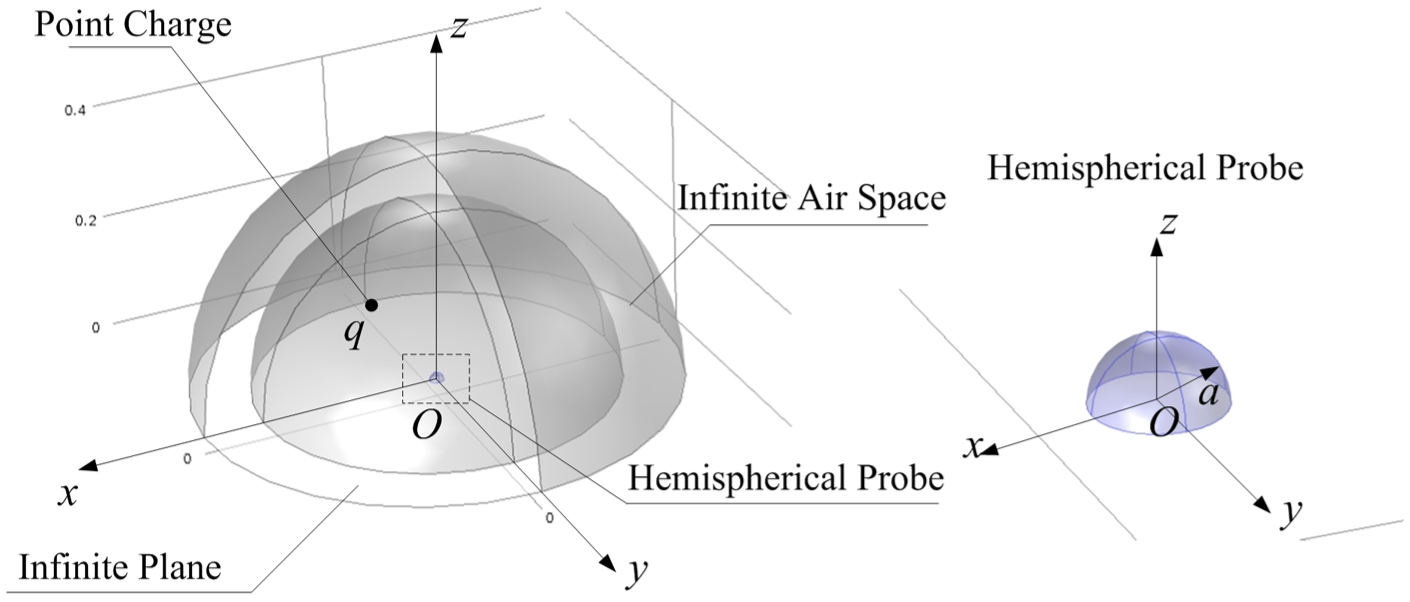
As shown in Figure 1, a hemisphere-shaped electrostatic sensor is installed on a pipeline. The sensor is mainly composed of a hemispherical probe, a dielectric layer, a shell, and a signal conditioner. The probe is inside the pipeline with its bottom face close to the pipelines inner wall ideally. When charged particles pass the pipeline, the electric field around the probe will fluctuate accordingly. Thus, there will be induced changing charges on the probe surface. It is noteworthy that the induced charges are weak and sensitive to external interferences, so they have to be converted into voltage signals immediately for post-processing by the signal conditioner. Consequently, the output signals of an electrostatic sensor are voltages instead of charges.

Figure 1.

Schematic diagram of a hemisphere-shaped electrostatic sensor installed on a pipeline.

As mentioned above, static sensitivity was used to describe the sensitivity characteristics of electrostatic sensors in previous studies.^3,11,31,32 It reflects a basic relationship between the static charged particles and the corresponding induced charges, on which the definition and analytical model of dynamic sensitivity will be based. Therefore, first of all, static sensitivity has to be studied.

An analytical model of hemisphere-shaped electrostatic sensors’ static sensitivity was provided in our previous work. ¹⁷ In the modeling, when calculating the total induced charges using the integral of charge density, an implied condition for determining the integrating range was not considered to obtain a concise model. However, it would influence the accuracy to some extent. Therefore, we will improve the model for a more accurate description of static sensitivity in this section.

Electrostatic field model in a grounded pipeline

As shown in Figure 1, a Descartes coordinate system is established with the center of the probe’s bottom face set as the origin. The axial direction of the pipeline and that of the probe were set as the x-axis and the z-axis, respectively, and then the y-axis is determined automatically. Thus, a point in the pipeline is denoted as $P(x,y,z)$ .

It is assumed that the volume charge density ${\rho }_t(P)$ is a prescribed function that describes different charge motions at time t, and ${\phi }_t(P)$ is the corresponding potential distribution in the pipeline. The interior area of the pipeline is denoted as V. The corresponding boundary is denoted as $\Gamma$ , which includes the probes hemispherical surface ${\Gamma }_1$ and the pipelines inner wall ${\Gamma }_2$ . Since the time $(10^{-19}\mathrm{s})$ to reach electrostatic equilibrium state is much shorter than the passing time of a charged particle, the interaction between the probe and moving charged particles can be described by pure electrostatic field.^3,17 And the field is determined by Poisson equation and Dirichlet boundary conditions uniquely as follows

$$\Delta {\phi }_t\left(P\right)=-\frac{{\rho }_t\left(P\right)}{\epsilon },s.t.\{\begin{array}{c}\phi \left(P\right)=0,P\in {\Gamma }_2\hfill \\ \phi \left(P\right)=\mathrm{cons}\left(t\right),P\in {\Gamma }_1\hfill \\ \underset{P\to \infty }{lim}\phi \left(P\right)=0\hfill \end{array}$$

(1)

where $\mathrm{cons}(t)$ is a constant function of t describing the equipotential surface of the probe, $\epsilon$ is the permittivity of free space, and $\Delta$ is the Laplace operator. Furthermore, the solution of the Poisson equation can be obtained using Green function as follows

$${\phi }_t\left(P\right)=\underset{V}{\int }G(P,P_0){\rho }_t\left(P_0\right)d{V}_0-\epsilon \underset{\Gamma }{\oint }{f}_t\left(P_0\right)\frac{\partial G(P,P_0)}{\partial {\stackrel{\rightharpoonup }{n}}_0}d{S}_0$$

(2)

where the volume charge density has been rewritten as ${\rho }_t(P_0)$ to be distinguished as an integral term, $f_t(P_0)$ denotes the potential distribution on $\Gamma$ at time t, $\partial /\partial {\stackrel{\rightharpoonup }{n}}_0$ represents the directional derivative in the exterior normal direction of $\Gamma$ , and $G(P,P_0)$ is the Green function that describes the potential distribution in V when a unit point charge is located at $P_0$ , and when the pipeline and the probe are both grounded. It is obvious that how to calculate the Green function is also a boundary value problem of the Poisson equation.

Solution of the Green function using the method of image charges

According to previous studies,^2,9,11 the electrostatic field on the inner wall of a pipeline is commonly simplified as that on an infinite plane when the dimension of the pipeline is much bigger than that of the probe. Under this case, the method of image charges can be used. That is to say, when a point charge $q_0$ is located at $P_0(x_0,y_0,z_0)$ , the corresponding induced charges on the boundary $\Gamma$ can be replaced by three image point charges located at $P_1,P_2,\mathrm{and}{P}_3$ , respectively, as shown in Figure 2.

Figure 2.

Schematic diagram of the method of image charges.

Here, the image point charges are denoted as $q_1,q_2,\mathrm{and}{q}_3$ , respectively. The radius of the probe is denoted as a and the distance from the origin to $P_0$ as b. Then, according to the method of image charges, the three image point charges are calculated as $q_1=-a{q}_0/b$ , $q_2=-q_0$ , and $q_3=a{q}_0/b$ , while their coordinates are $(a^2{x}_0/b^2,a^2{y}_0/b^2,a^2{z}_0/b^2)$ , $(x_0,y_0,-z_0)$ , and $(a^2{x}_0/b^2,a^2{y}_0/b^2,-a^2{z}_0/b^2)$ , respectively. In this way, the potential distribution in V generated by the point charge and the three image charges is consistent with that by the point charge and the actual induced charges on the boundary. Therefore, when $q_0=1\mathrm{C}$ , the potential at an arbitrary point $P(x,y,z)$ is determined by equation (3) according to the superposition principle of electrostatic field

$$G(P,P_0)=\frac{1}{4\pi \epsilon }(\frac{1}{\left|P{P}_0\right|}-\frac{1}{\left|P{P}_2\right|}-\frac{a}{b\left|P{P}_1\right|}+\frac{a}{b\left|P{P}_3\right|})$$

(3)

More details about the above modeling steps can be found in our previous work. ¹⁷

Improved analytical model of static sensitivity

Next, the total induced charges on the probe will be calculated using the integral of charge density. In our previous work, ¹⁷ an implied condition for determining the integrating range was not considered, so the model is less accurate. Thus, it will be improved in the following.

According to the relationship between the charge density on a conductor surface and surrounding potential distribution, the charge density ${\sigma }_t(P)$ at $P(x,y,z)$ on $\Gamma$ is derived from equation (2)

$$\begin{array}{cc}\multicolumn{1}{c}{{\sigma }_t\left(P\right)}& =\epsilon \frac{\partial {\phi }_t\left(P\right)}{\partial \stackrel{\rightharpoonup }{n}}\hfill \\ \multicolumn{1}{c}{}& =\epsilon \underset{V}{\int }\frac{\partial G(P,P_0)}{\partial \stackrel{\rightharpoonup }{n}}{\rho }_t\left(P_0\right)d{V}_0-{\epsilon }^2\underset{\Gamma }{\oint }{f}_t\left(P_0\right)\frac{\partial \left(\frac{\partial G(P,P_0)}{\partial \stackrel{\rightharpoonup }{n}}\right)}{\partial {\stackrel{\rightharpoonup }{n}}_0}d{S}_0\hfill \end{array}$$

(4)

where $\partial /\partial \stackrel{\rightharpoonup }{n}$ represents the directional derivative in the inner normal direction of $\Gamma$ . Supposing that there is only one point charge $q_0$ located at $P_0$ , the induced charge on the probe can be calculated as follows using the integral of ${\sigma }_t(P)$ on the hemispherical surface ${\Gamma }_1$ , that is to say

$$Q_{{\Gamma }_1}=\epsilon q_0\underset{{\Gamma }_1}{\int }\frac{\partial G(P,P_0)}{\partial \stackrel{\rightharpoonup }{n}}\mathrm{dS}-\mathrm{cons}\left(t\right)\lambda$$

(5)

where $\lambda =-{\epsilon }^2{\int }_{{\Gamma }_1}\partial {\int }_{{\Gamma }_1}(\partial G(P,P_0)/\partial \stackrel{\rightharpoonup }{n})d\mathrm{S}/\partial {\stackrel{\rightharpoonup }{n}}_{0}d{S}_0$ is the capacitance of the probe itself. ¹⁷ It can be derived using Gauss’ law that $\lambda =2\pi a\epsilon$ is a constant. Because $\lambda$ is quite small (10⁻¹³) and $\mathrm{cons}(t)$ is also a small value,^10,21 and the second term on the right side of equation (5) can be ignored. Thus, the induced charge on the probe is simplified as

$$Q_{{\Gamma }_1}=\epsilon q_0\underset{{\Gamma }_1}{\int }\frac{\partial G(P,P_0)}{\partial \stackrel{\rightharpoonup }{n}}\mathrm{dS}$$

(6)

However, it is difficult to calculate the directional derivative in equation (6) because the direction of $\stackrel{\rightharpoonup }{n}$ changes with P. To solve this problem, an integral conversion strategy is adopted in the following.

First, the induced charges on the whole boundary $\Gamma$ and that on the inner wall ${\Gamma }_2$ are denoted by $Q_{\Gamma }$ and $Q_{{\Gamma }_2}$ , respectively. Since the length of the pipeline is much longer than the radius, it can be assumed that all the electric field lines end in the pipeline. Therefore, the total induced charges on $\Gamma$ will be $-q_0$ when a point charge $q_0$ is present in the pipeline according to Gauss’ law. That is to say

$$Q_{\Gamma }=Q_{{\Gamma }_1}+Q_{{\Gamma }_2}=-q_0$$

(7)

Since ${\Gamma }_2$ is simplified as an infinite plane, the potential distribution in V can be equivalently represented by that generated by the point charge and its three image point charges. Now, if we replace ${\Gamma }_1$ by a round plane ${\Gamma }_{\mathrm{C}}$ , then ${\Gamma }_2$ and ${\Gamma }_{\mathrm{C}}$ will make up a complete plane ${\Gamma }_{\mathrm{P}}$ . Under this case, the total charge on ${\Gamma }_{\mathrm{P}}$ is

$$Q_{{\Gamma }_{\mathrm{P}}}=Q_{{\Gamma }_{\mathrm{C}}}+Q_{{\Gamma }_2}=-(q_0+q_1)$$

(8)

Then, we will have

$$Q_{{\Gamma }_2}=Q_{{\Gamma }_{\mathrm{P}}}-Q_{{\Gamma }_{\mathrm{C}}}=-(q_0+q_1)-Q_{{\Gamma }_{\mathrm{C}}}$$

(9)

Next, by substituting equation (9) into equation (7), we will obtain

$$Q_{{\Gamma }_1}=-q_0-(-q_0-q_1+Q_{{\Gamma }_{\mathrm{C}}})=q_1-Q_{{\Gamma }_{\mathrm{C}}}$$

(10)

where $q_1=-a{q}_0/b$ . Thus, the integral on ${\Gamma }_1$ in equation (6) can be replaced by that on ${\Gamma }_{\mathrm{C}}$ . The advantage of this way is that calculation of the directional derivative is simplified significantly because the potential near ${\Gamma }_{\mathrm{C}}$ is zero except that in the z-direction. Thus, equation (6) will be transformed into equation (11)

$$Q_{{\Gamma }_1}=-\frac{a{q}_0}{b}-\epsilon q_0\underset{{\Gamma }_{\mathrm{C}}}{\int }\frac{\partial G(P,P_0)}{\partial z}\mathrm{dS}$$

(11)

Furthermore, by substituting equation (3) into equation (11), while calculating the integrals in polar coordinates, then, one will have

$$\begin{array}{c}{Q}_{{\Gamma }_1}=-\frac{a{q}_0}{b}-\frac{z_0{q}_0}{2\pi }\underset{0}{\overset{2\pi }{\int }}d\theta \underset{0}{\overset{a}{\int }}{[{(r\cos \theta -x_0)}^2+{(r\sin \theta -y_0)}^2+z_0^2]}^{-\frac{3}{2}}\mathrm{rdr}\hfill \\ +\frac{a^3{z}_0{q}_0}{2\pi b^3}\underset{0}{\overset{2\pi }{\int }}d\theta \underset{0}{\overset{a}{\int }}{[{(r\cos \theta -\frac{a^2{x}_0}{b^2})}^2+{(r\sin \theta -\frac{a^2{y}_0}{b^2})}^2+\frac{a^4{z}_0^2}{b^4}]}^{-\frac{3}{2}}\mathrm{rdr}\hfill \end{array}$$

(12)

Next, according to previous studies,^3,11,31,32 the electrostatic sensor’s static sensitivity at $P(x,y,z)$ is defined as

$$S(x,y,z)=\left|\frac{Q}{q}\right|$$

(13)

where q is a point charge located at $P(x,y,z)$ and Q is the corresponding induced charges on the probe. Finally, based on equations (12) and (13), the static sensitivity of a hemisphere-shaped electrostatic sensor is expressed as

$$\begin{array}{c}\multicolumn{1}{c}{S(x,y,z)=\frac{a}{b}+\frac{z}{2\pi }\underset{0}{\overset{2\pi }{\int }}d\theta \underset{0}{\overset{a}{\int }}{[{(r\cos \theta -x)}^2+{(r\sin \theta -y)}^2+z^2]}^{-\frac{3}{2}}\mathrm{rdr}}\\ \multicolumn{1}{c}{=-\frac{a^{3}z}{2\pi b^3}\underset{0}{\overset{2\pi }{\int }}d\theta \underset{0}{\overset{a}{\int }}{[{(r\cos \theta -\frac{a^{2}x}{b^2})}^2+{(r\sin \theta -\frac{a^{2}y}{b^2})}^2+\frac{a^4{z}^2}{b^4}]}^{-\frac{3}{2}}\mathrm{rdr}}\end{array}$$

(14)

Moreover, since the hemispherical probe and the boundary condition are both symmetric with the z-axis, it is obvious that S is also symmetric with the z-axis. Therefore, $S(x,y,z)$ can be expressed as follows

$$\begin{array}{c}S(b,\beta )=\frac{a}{b}+\hfill \\ \frac{b\cos \beta }{2\pi }\underset{0}{\overset{2\pi }{\int }}d\theta \underset{0}{\overset{a}{\int }}{[{\left(r\cos \theta \right)}^2+{(r\sin \theta -b\sin \beta )}^2+b^2{\cos }^2\beta ]}^{-\frac{3}{2}}\mathrm{rdr}\hfill \\ -\frac{a^3\cos \beta }{2\pi b^2}\underset{0}{\overset{2\pi }{\int }}d\theta \underset{0}{\overset{a}{\int }}{[{\left(r\cos \theta \right)}^2+{(r\sin \theta -\frac{a^2}{b}\sin \beta )}^2+\frac{a^4}{b^2}{\cos }^2\beta ]}^{-\frac{3}{2}}\mathrm{rdr}\hfill \end{array}$$

(15)

where $\beta$ is the included angle between the line OP and the z-axis. Compared to the model in our previous work, ¹⁷ it can be easily found that two integral terms are added, which makes a more accurate description of the sensor’s static sensitivity.

As mentioned above, it is noteworthy that static sensitivity reflects the relationship between static charged particles and the induced charges. However, the charged particles are always moving in most practical applications, so the induced charges on the probe change continuously. Besides, the output signals of an electrostatic sensor are not charge signals but voltage ones transformed by the signal conditioner. In addition, static sensitivity is defined in the three-dimensional space, which makes it difficult to build a unified analytical model if the actual pipeline shape is considered; however, not all the signals from the whole space are important in practice. Thus, static sensitivity is not direct, accurate, and practical for applications that detect moving particles.

Theoretical analysis of hemisphere-shaped electrostatic sensors’ dynamic sensitivity

To overcome the drawbacks of static sensitivity, dynamic sensitivity is proposed in this section, which is defined based on the static sensitivity.

Output voltage signals of hemisphere-shaped electrostatic sensors

It is assumed that charged particles move along the pipeline’s axial direction at a constant velocity.^4,10,13 Thus, the changes in the induced charges on the probe can be calculated by static sensitivity at evenly spaced points. Furthermore, the output voltage signals are obtained from the signal conditioner.

First, it is supposed that a charged particle q moves along the pipeline’s axial direction at a velocity of v, as shown in Figure 1. Thus, its y-coordinates and z-coordinates can be regarded as constants, while its x-coordinates can be expressed using a form related to v and t, that is, $x=x_0+\mathrm{vt}$ , where $x_0$ is the initial position of the particle. Thus, the time-varying induced charge signal is expressed as follows

$$Q\left(t\right)=-q{S}_{y,z}(x_0+\mathrm{vt})$$

(16)

where $S_{y,z}(x_0+\mathrm{vt})$ denotes the static sensitivity when the y-coordinates and the z-coordinates of the particle are regarded as constants. In this article, for the convenience of signal analysis, the signal conditioner is designed as a proportional two-stage amplifier which is mainly composed of two operational amplifiers, as shown in Figure 3. The first stage is a charge–voltage conversion circuit which transforms the induced charge into voltage proportionally. The second stage is a voltage amplifier circuit which amplifies the transformed voltage to a magnitude for post-processing.

Figure 3.

Schematic diagram of the signal conditioner.

It is obvious that the total function of the signal conditioner can be represented by an amplification coefficient K whose unit is $\mathrm{V}/\mathrm{C}$ . Then, the output signal is expressed as equation (17)

$$u\left(t\right)=-\mathrm{qK}{S}_{y,z}(x_0+\mathrm{vt})$$

(17)

Finally, combining equations (17) and (15), one can obtain

$$\begin{array}{c}u\left(t\right)=-\frac{\mathrm{aqK}}{b}-\frac{\mathrm{bqK}\cos \beta }{2\pi }\hfill \\ \underset{0}{\overset{2\pi }{\int }}d\theta \underset{0}{\overset{a}{\int }}{[{(r\cos \theta -b\sin \beta )}^2+r^2{\cos }^2\theta +b^2{\cos }^2\beta ]}^{-\frac{3}{2}}\mathrm{rdr}\hfill \\ +\frac{a^3\mathrm{qK}\cos \beta }{2\pi b^2}\hfill \\ \underset{0}{\overset{2\pi }{\int }}d\theta \underset{0}{\overset{a}{\int }}{[{(r\cos \theta -\frac{a^2}{b}\sin \beta )}^2+r^2{\cos }^2\theta +\frac{a^4}{b^2}{\cos }^2\beta ]}^{-\frac{3}{2}}\mathrm{rdr}\hfill \end{array}$$

(18)

where the coefficient $b=\sqrt{{(x_0+\mathrm{vt})}^2+y^2+z^2}$ and $\beta =\arctan (\sqrt{{(x_0+\mathrm{vt})}^2+y^2}/z)$ . It is clear that $u(t)$ is proportional to q and K. For the sake of simplicity, here, we set $K=1$ , $q=-1\mathrm{C}$ , and the time when the particle reaches the cross section $x=0$ is set as the zero time. Then, the output voltage signals of hemisphere-shaped electrostatic sensors can be easily calculated by equation (18). Figure 4 shows the output voltage signals when the motion paths z-coordinates are set to 50 mm; the y-coordinates are set to 0, 10, 20, 30, 40, and 50 mm, respectively; and the velocities of the charged particle are set to 1, 2, and 3 m/s, respectively.

Figure 4.

The output voltage signals of the hemisphere-shaped electrostatic sensor.

It can be seen that, first, all of the peaks $u_{max}$ appear when the charged particle reaches the cross section of $x=0$ . Second, when q is set as a constant, the values of $u_{max}$ are just related to the coordinates in the cross section but has nothing to do with velocity. In addition, it is convenient for us to observe and obtain the values of the peaks in practice. Thus, the peaks $u_{max}$ are quite appropriate for us to study the practical sensitivity of electrostatic sensors that detect moving charged particles. Here, we call the plane $x=0$ as the observation cross section, in which the direct relationship between the charge q, the corresponding signal peak $u_{max}$ , and the motion path’s coordinates $(y,z)$ can be built easily and sensitively. Consequently, dynamic sensitivity is defined within the observation cross section.

Definition of dynamic sensitivity

According to the above analysis, dynamic sensitivity $S_D$ is defined within the observation cross section to establish a direct relationship between the moving charged particles and the corresponding output voltage signals.

The peak along an arbitrary motion path $(y,z)$ is expressed as $u_{max}=-\mathrm{qK}{S}_{y,z}(0)$ according to equation (17), which can be rewritten as $u_{max}(y,z)=-\mathrm{qK}{S}_{x=0}(y,z)$ for a more visualized form. Then, dynamic sensitivity is defined as the absolute value of the output voltage signal’s peak from a moving unit point charge, which is expressed as follows

$$S_D(y,z)=\left|\frac{-\mathrm{qK}{S}_{x=0}(y,z)}{q}\right|=K{S}_{x=0}(y,z)$$

(19)

Furthermore, by substituting equation (14) into equation (19), we can obtain

$$\begin{array}{c}{S}_D(b,\beta )=\frac{\mathrm{aK}}{b}+\frac{\mathrm{bK}\cos \beta }{2\pi }\hfill \\ \underset{0}{\overset{2\pi }{\int }}d\theta \underset{0}{\overset{a}{\int }}{[{\left(r\cos \theta \right)}^2+{(r\sin \theta -b\sin \beta )}^2+b^2{\cos }^2\beta ]}^{-\frac{3}{2}}\mathrm{rdr}\hfill \\ -\frac{a^{3}K\cos \beta }{2\pi b^2}\hfill \\ \underset{0}{\overset{2\pi }{\int }}d\theta \underset{0}{\overset{a}{\int }}{[{\left(r\cos \theta \right)}^2+{(r\sin \theta -\frac{a^2}{b}\sin \beta )}^2+\frac{a^4}{b^2}{\cos }^2\beta ]}^{-\frac{3}{2}}\mathrm{rdr}\hfill \end{array}$$

(20)

where $b=\sqrt{y^2+z^2}$ and $\beta =\arctan (y/z)$ .

By comparing the definition of dynamic sensitivity with that of static sensitivity, it is clear that dynamic sensitivity reflects a direct and optimized relationship between moving charged particles and corresponding output voltage signals, which has nothing to do with velocity, while static sensitivity reflects a relationship between static charged particles and corresponding induced charges. Thus, as for moving charged particles, dynamic sensitivity is much more visualized, reasonable, and concise than static sensitivity. In addition, dynamic sensitivity is defined in a specific plane, while static sensitivity is defined in the three-dimensional space. Thus, if boundary conditions are not axisymmetric in the space just as most applications, it is difficult to build a unified analytical model of static sensitivity, but it is still likely to obtain a unified analytical model of dynamic sensitivity. In a word, dynamic sensitivity has overcome the drawbacks of static sensitivity and is direct and practical for applications that detect moving particles.

Calibration method of dynamic sensitivity under actual boundary conditions

It is noteworthy that the definition of dynamic sensitivity as equation (20) is based on the common simplified boundary condition that the pipeline’s inner wall ${\Gamma }_2$ is simplified as an infinite plane. However, an electrostatic sensor is usually installed on a grounded pipeline in practice, and the probe’s bottom face cannot contact the pipeline due to insulation. Therefore, the actual electrostatic field will be different from that under the simplified boundary condition. Consequently, the actual dynamic sensitivity will be different from that described by equation (20) to some extent.

To improve the accuracy of the analytical model under actual boundary conditions, a promising method is adding a calibration item $R(b,\beta )$ into the uncalibrated model $S_D(b,\beta )$ according to the actual boundary condition. Then, a calibrated model $S_{\mathrm{RD}}(b,\beta )$ is expressed as

$$S_{\mathrm{RD}}(b,\beta )=S_D(b,\beta )R(b,\beta )$$

(21)

where the calibration item $R(b,\beta )$ is calculated in the following.

First, grid points are chosen in the observation cross section. They should cover almost the whole section. Then, values of the uncalibrated analytical dynamic sensitivity are calculated by equation (20) at the points. Next, an FEM simulation model is built to emulate the actual boundary condition, by which values of the simulated dynamic sensitivity are obtained at the points. Finally, the ratios of the simulated dynamic sensitivity to the uncalibrated one are calculated at the grid points, and $R(b,\beta )$ is obtained by fitting the ratios with b and $\beta$ .

To ensure the accuracy of the calibrated model, first, the uncalibrated model has to be accurate under the common simplified boundary condition. Second, the FEM simulation model also has to be accurate. Moreover, a high fitting precision is also indispensable in calculating $R(b,\beta )$ . These conditions will be validated in section “Simulation-based validations.”

Simulation-based validations

Validations of the uncalibrated model of dynamic sensitivity

As mentioned before, the uncalibrated model as equation (20) is based on the common simplified boundary condition that the pipelines inner wall ${\Gamma }_2$ is simplified as an infinite plane. Accordingly, an FEM simulation model is built. As shown in Figure 5, an infinite plane fitted with a hemispherical probe is modeled in COMSOL. The probe is 12 mm in radius and surrounded by an infinite airspace. Boundary conditions are set to ground for the plane and the probe. The airspace is assumed to have a relative dielectric constant of 1. A single charged particle modeled as a point charge is then added.

Figure 5.

The FEM simulation model under the simplified boundary condition.

A free tetrahedral mesh strategy is used. In order to ensure a mesh convergence and a high accuracy of the FEM model, on one hand, some tiny structures of the electrostatic sensor were simplified. They have negligible impact on the simulated results, but they generate tiny and abnormal meshes that have low quality. On the other hand, the meshes were refined where the electrostatic field varies intensely, such as the meshes near the point charge and the hemispherical probe. Approximately 30,000 elements are generated as shown in Figure 6.

Figure 6.

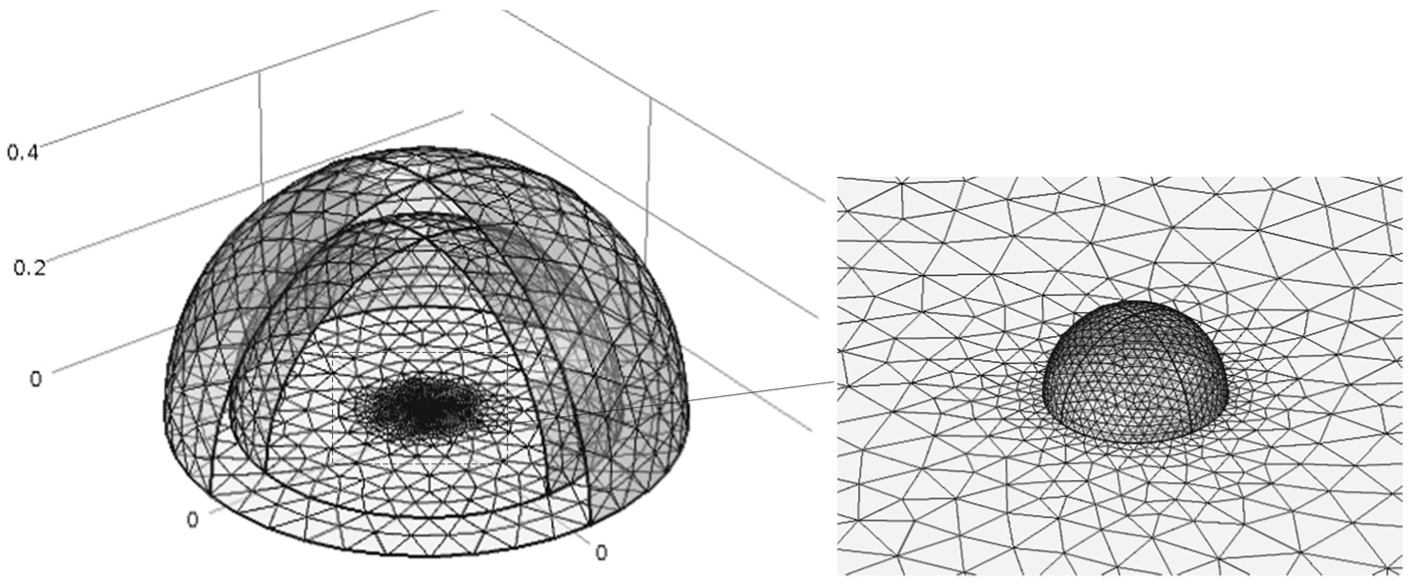
Free tetrahedral meshing of the FEM simulation model.

For the sake of simplicity, here, we set the amplification coefficient $K=1$ and the point charge $q=-1\mathrm{C}$ . Then, it is easy to know that the total induced charge on the probe equals to dynamic sensitivity numerically. Next, according to the symmetry of the probe and the boundary condition, grid points are chosen in the $x=0$ plane, as shown in Figure 7. They are representative because they have covered a wide fan-shaped area which has a radius of 200 mm and an included angle of ${170}^{\circ }$ . Then, the corresponding values of dynamic sensitivity are calculated at the points by equation (20) and the FEM simulation model, respectively.

Figure 7.

The grid points in the $x=0$ plane.

Surface diagrams of the uncalibrated analytical dynamic sensitivity and the simulated one are shown in Figure 8, and the contour ones are shown in Figure 9. It is obvious that the analytical result is highly consistent with the simulated result. Further analysis shows that the mean absolute value of relative error from all the grid points is just 0.795%, which can be explained by analytical error of finite element.

Figure 8.

(a) Surface diagram of the uncalibrated analytical dynamic sensitivity and (b) surface diagram of the simulated dynamic sensitivity.

Figure 9.

(a) Contour diagram of the uncalibrated analytical dynamic sensitivity and (b) contour diagram of the simulated dynamic sensitivity.

Conclusions are drawn from the close agreement between the two sets of results that the uncalibrated model of dynamic sensitivity as equation (20) is accurate under the common simplified boundary condition. Conversely, the accuracy of the FEM simulation method has been validated, which offers confidence that results from an FEM simulation model can be used to calibrate the uncalibrated model under actual boundary conditions.

Validations of the calibration method and the calibrated model of dynamic sensitivity

Comparisons between the uncalibrated model and FEM simulation model

A circular pipeline with a radius of 200 mm and a length of 1 m is considered here. Accordingly, an FEM simulation model is built. As shown in Figure 10, a pipeline fitted with a hemispherical probe is modeled in COMSOL. Similarly, the probe is 12 mm in radius and surrounded by an airspace. However, there is a distance of 2 mm between its bottom face and the pipeline’s inner wall. Other conditions are set the same as the model shown in Figure 5. Moreover, a similar free tetrahedral mesh strategy is used, and approximately 110,000 elements were generated.

Figure 10.

The FEM simulation model under the actual boundary condition.

Similarly, we set $K=1$ and $q=-1\mathrm{C}$ for the sake of simplicity. Then, the total induced charge is equal to the dynamic sensitivity numerically, when the point charge is placed in the observation cross section. Accordingly, grid points are chosen in that section, as shown in Figure 11. They are representative because they have covered almost the whole observation cross section, and denser points are set near the probe for a better description of the fast-changing dynamic sensitivity in that area. Then, the corresponding values of dynamic sensitivity are calculated at the points by equation (20) and the FEM simulation model, respectively.

Figure 11.

The grid points in the observation cross section.

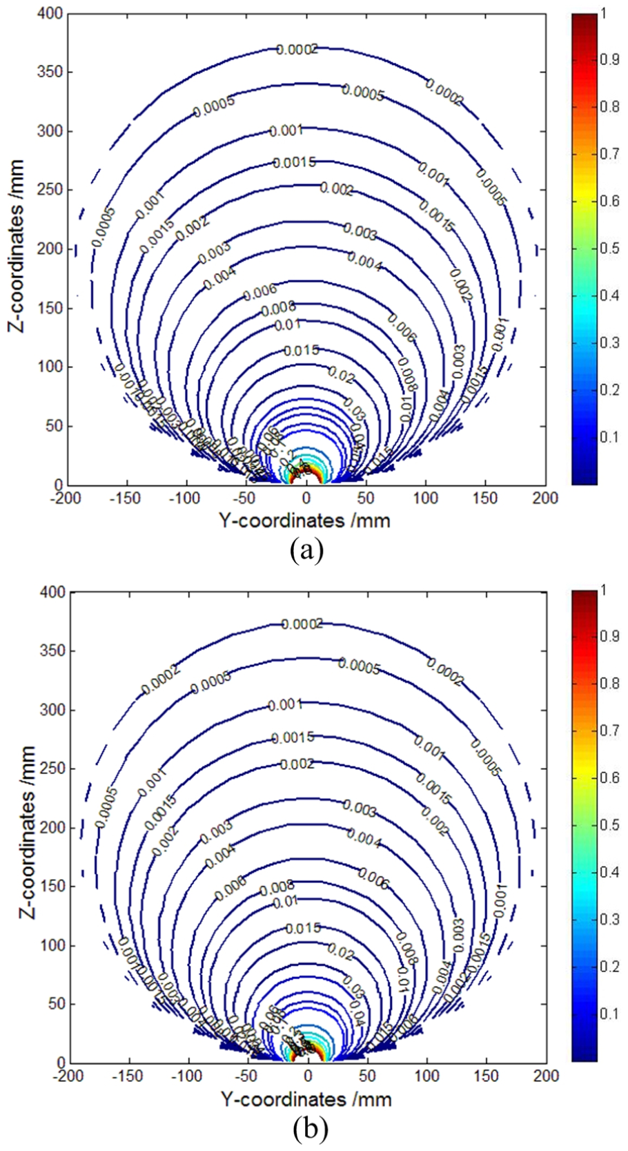
Contour diagrams of the uncalibrated analytical dynamic sensitivity and the simulated one in the observation cross section are shown in Figure 12. And the relative error between the simulated and the uncalibrated analytical dynamic sensitivity is shown in Figure 13.

Figure 12.

(a) Contour diagram of the uncalibrated analytical dynamic sensitivity and (b) contour diagram of the simulated dynamic sensitivity.

Figure 13.

Relative error between the simulated and the uncalibrated analytical dynamic sensitivity.

It is observed from Figures 12 and 13 that the uncalibrated analytical result is consistent with the simulated one from the viewpoint of general distribution trend because all of the contour lines of dynamic sensitivity are fan-shaped distributed and oriented from the origin. Thus, the uncalibrated model has provided a valid infrastructure to describe dynamic sensitivity. In addition, from the viewpoint of numerical contrast, the uncalibrated analytical result and the simulated one are similar near the probe generally. Then, the simulated result decreases faster than the analytical one with the increase in b, leading to the maximal relative error near the pipeline’s inner wall. Also, the error gradient varies with the included angles $\beta$ shown in Figure 11. Thus, b and $\beta$ can be used to fit the relative error and construct the calibration item. Besides, it is seen that there exists an obvious relative error in the side of the probe, which is caused by the distance between the probe’s bottom face and the pipeline’s inner wall. Since the corresponding area is quite small compared with the whole cross section, the error can be ignored for better conciseness and accuracy of the calibration item from a general view.

Calculation of the calibration item

According to the calibration method proposed in section “Calibration method of dynamic sensitivity under actual boundary conditions,” first, grid points are chosen in the observation cross section, as shown in Figure 11. Then, values of the uncalibrated analytical dynamic sensitivity and the simulated dynamic sensitivity are calculated, as shown in Figure 12(a) and (b), respectively. Next, ratios of the simulated dynamic sensitivity to the uncalibrated one are calculated at the points. Afterward, on the lines of different $\beta$ shown in Figure 11, a power function model as equation (22) is used to fit the relationship between the ratios and b

$$R\left(b\right)=p_1{b}^{p_2}+p_3$$

(22)

where $p_1,p_2,\mathrm{and}{p}_3$ are the fitting parameters. In practice, the whole cross section is divided into two areas: $b\ge D$ and $b<D$ , as shown in Figure 14, where D is determined according to the variation trend of the radios, and it is fitted as $D=-0.0188\beta +0.0444$ . It is seen that the relative error in the area of $b<D$ is relatively small. In addition, the area is quite small compared with the whole section. Thus, the ratios are only fitted in the area of $b\ge D$ to obtain a higher fitting precision from a general view.

Figure 14.

(a) The fitting area $(b\ge D)$ and the ignored area $(b<D)$ and (b) relative error in the ignored area $(b<D)$ .

The fitted result of the relationship between the ratios and b is shown in Figure 15, where each curve represents one fitting function of the corresponding $\beta$ . It is seen that the fitted curves are highly coincident with the fitting points, and further analysis shows that the mean absolute value of relative error from all the fit points is just 1.96%. Thus, a high fitting precision is obtained.

Figure 15.

The fitted result between the ratios and b on the lines of different $\beta$ .

Next, a binomial Gaussian function model as equation (23) is used to fit the relationships between $\beta$ and $p_1,p_2,\mathrm{and}{p}_3$ in equation (22)

$$P\left(\beta \right)=a{e}^{n{\beta }^2}+c{e}^{d{\beta }^2}$$

(23)

where $a,n,c,\mathrm{and}d$ are the fitting parameters. The fitted results of $p_1$ , $p_2$ , and $p_3$ are shown in Figure 16. It is seen that the fitted curves are highly coincident with the fitting points in each diagram, and further analysis shows that the mean absolute values of relative error are 0.68%, 0.37%, and 0.76%, respectively. Thus, a high fitting precision is obtained.

Figure 16.

The fitted results (a) between $\beta$ and $p_1$ , (b) between $\beta$ and $p_2$ , and (c) between $\beta$ and $p_3$ .

Finally, the calibration item $R(b,\beta )$ is expressed as follows

$$R(b,\beta )=\{\begin{array}{cc}{p}_1{b}^{p_2}+p_3,\hfill & \mathrm{if}b\ge D\hfill \\ \multicolumn{1}{c}{1,}& \mathrm{if}b<D\hfill \end{array}$$

(24)

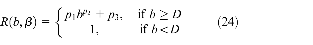
where

$$\{\begin{array}{c}{p}_1=-5.7311\times {10}^{-8}{e}^{8.7639{\beta }^2}-6.103e^{0.5724{\beta }^2}\hfill \\ p_2=-43.9996e^{0.1261{\beta }^2}+45.9113e^{0.113{\beta }^2}\hfill \\ p_3=1.0479e^{7.0643\times {10}^{-2}{\beta }^2}+1.2218\times {10}^{-4}{e}^{4.4059{\beta }^2}\hfill \end{array}$$

(25)

The calibrated model of dynamic sensitivity

By substituting equation (24) into equation (21), the calibrated model of dynamic sensitivity is expressed as follows

$$S_{\mathrm{RD}}(b,\beta )=\{\begin{array}{cc}{S}_D(b,\beta )(p_1{b}^{p_2}+p_3),\hfill & \mathrm{if}b\ge D\hfill \\ \multicolumn{1}{c}{S_D(b,\beta ),}& \mathrm{if}b<D\hfill \end{array}$$

(26)

where the function of $S_{\mathrm{RD}}$ can be found in equation (20) and functions of $p_1$ , $p_2$ , and $p_3$ can be found in equation (25). The contour diagrams of the calibrated analytical dynamic sensitivity and the simulated one are shown in Figure 17. The relative error between the simulated and the calibrated analytical dynamic sensitivity is shown in Figure 18.

Figure 17.

(a) Contour diagram of the calibrated analytical dynamic sensitivity and (b) contour diagram of the simulated dynamic sensitivity.

Figure 18.

The relative error between the simulated and the calibrated analytical dynamic sensitivity.

Comparing Figure 12 with Figure 17, it is observed that the analytical dynamic sensitivity becomes highly consistent with the simulated one after calibration. Furthermore, by comparing Figure 13 with Figure 18, it is observed that the relative error between the simulated and the analytical dynamic sensitivity has decreased significantly after calibration, only that there still exists a relative error of about 10% near the inner wall of the pipeline. This is because the values of dynamic sensitivity are quite small near the inner wall of the pipeline, so a very small difference in value will cause an obvious difference in relative error. It is concluded that the calibrated model describes dynamic sensitivity with high accuracy, when the hemisphere-shaped electrostatic sensor is installed on a grounded circular pipeline. Besides, the calibration method proposed in this article is practicable, which provides a feasible way to promote the results in this article to researches and applications under different boundary conditions.

For a more visualized observation of the calibrated analytical dynamic sensitivity, its surface diagram is shown in Figure 19. It is observed that the dynamic sensitivity of a hemisphere-shaped electrostatic sensor distributes highly inhomogeneous. In detail, when $K=1$ , the largest value of dynamic sensitivity is close to 1, which appears nearby the probe surface. Then, the dynamic sensitivity decreases sharply with the increase in distance around the probe. After that, it decreases much flatter and comes close to 0 nearby the inner wall of the pipeline. In a word, the values and the gradients of dynamic sensitivity are much larger around the hemispherical probe than those in the distance, which indicates localized sensing characteristics. Consequently, it suggests that hemisphere-shaped electrostatic sensors are suitable for electrostatic sensor arrays and electrostatic tomography systems to obtain multi-localized and multi-layered information.

Figure 19.

The surface diagram of the calibrated analytical dynamic sensitivity.

Conclusion

An accurate analytical model of hemisphere-shaped electrostatic sensor’s static sensitivity was built; based on it, dynamic sensitivity was defined and analyzed theoretically. Dynamic sensitivity reflects a more direct and optimized relationship between moving particles and an electrostatic sensor’s output voltage signals, and it is easier to build a unified analytical model. Consequently, it has overcome the drawbacks of static sensitivity and is direct and practical to be used for applications that detect moving particles. Moreover, it has been validated by the FEM simulations that the analytical model built in this article provides a valid infrastructure to describe the dynamic sensitivity of hemisphere-shaped electrostatic sensors under a common simplified boundary condition. And it can be adjusted by the calibration method to actual boundary conditions. Besides, the dynamic sensitivity indicates localized sensing characteristics of hemisphere-shaped electrostatic sensors. It is concluded as follows:

1. Compared with static sensitivity, dynamic sensitivity is more practical to describe the sensitivity characteristics, which offers better guidelines for electrostatic sensors’ design and utilizations.

2. The analytical models and the calibration method provide valid references for further researches and applications under different boundary conditions.

3. Hemisphere-shaped electrostatic sensors have localized sensing characteristics, which makes them suitable for applications that require multi-localized and multi-layered information.