Coordinated motion control model of a six-wheeled rocker lunar rover

Abstract

At present, control methods of the six-wheeled rocker lunar rover primarily consist of setting the same driving parameters for each wheel. This type of control method ignores the multiple active driving characteristics of the lunar rover and causes parasitic power loss. The main cause of the parasitic power loss is the uncoordinated motion of the driving elements. Therefore, in this article, a coordinated motion programming model of the six-wheeled rocker lunar rover based on the velocity projection theorem, the quasi-static mechanical model, and the rated power of the motor is established to eliminate parasitic loss, reduce driving energy, and improve energy efficiency. The analytical solution of the programming model based on the Kuhn–Tucker condition is also calculated. The coordinated motion control model saves energy, and it is suitable for other wheeled-type planet rovers. This model provides technical support for reducing the energy consumption of planet rovers.

Introduction

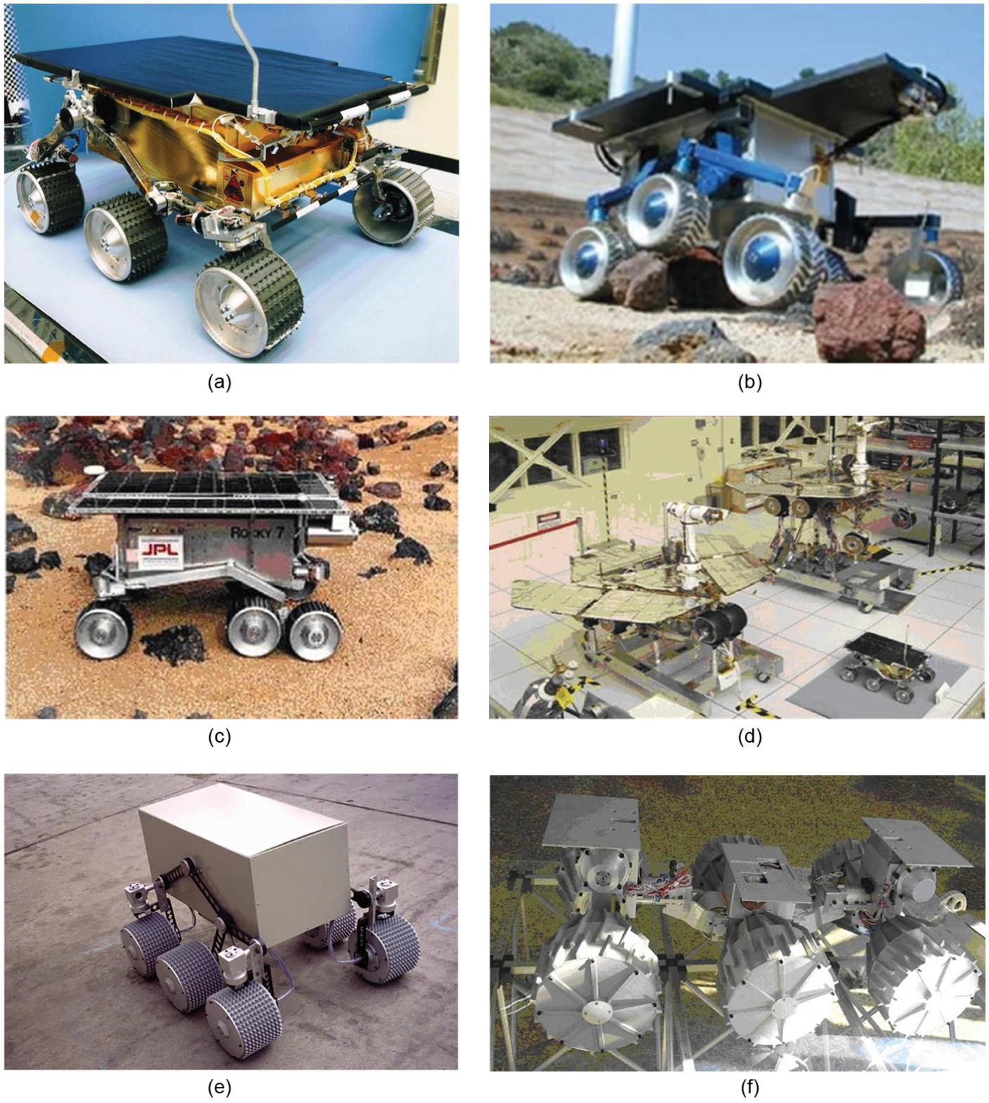
With the development of deep-space exploration technology, the moon has become the focus of deep-space exploration since the 1990s because of its abundant natural resources and advantages in astronomical observations. ¹ The primary method used to learn about the moon is lunar exploration with a lunar rover. Many countries have carried out the development of planet rovers and their control modes. These planet rovers are shown in Figure 1, and their motion control technologies are shown in Table 1.

Figure 1.

Planet rovers: (a) Sojourner Martian rover, ² (b) SDM prototype device, ³ (c) Rocky 7 prototype device,^4,5 (d) Spirit Martian rover, ⁶ (e) six-wheeled rocker lunar rover, ⁷ and (f) six cylinder-conical wheeled lunar rover. ⁸

Table 1.

Motion control technologies of planet rovers.

Rover or prototype device	Motion control technologies
Sojourner	Equipped with optical encoders, angle sensors, and gyroscopes; voltage control in the voltage relay for motor control; adopted teleoperation and local autonomous navigation mode for navigation and motion control; adopted behavior control for obstacle avoidance
SDM	Equipped with brush motors, encoders, angle sensors, inertial measurement units, three pairs of visual cameras and FPGA motor controller; software structure based on the task model
Rocky 7	Equipped with navigation cameras; rover guidance to a particular direction using course information with autonomous obstacle avoidance
Spirit	Equipped with encoders, potentiometers, and gyroscopes; motor control by PWM servo control in speed mode; HBUS based on VME; VxWorks-embedded operating system; layered software architecture; human–computer interaction, and autonomous navigation mode
Six-wheeled rocker lunar rover	Equipped with sensors; passively controlled to adapt to the terrain
Six cylinder-conical wheeled lunar rover	Equipped with servo control cards and motors; adaptive drive control algorithm

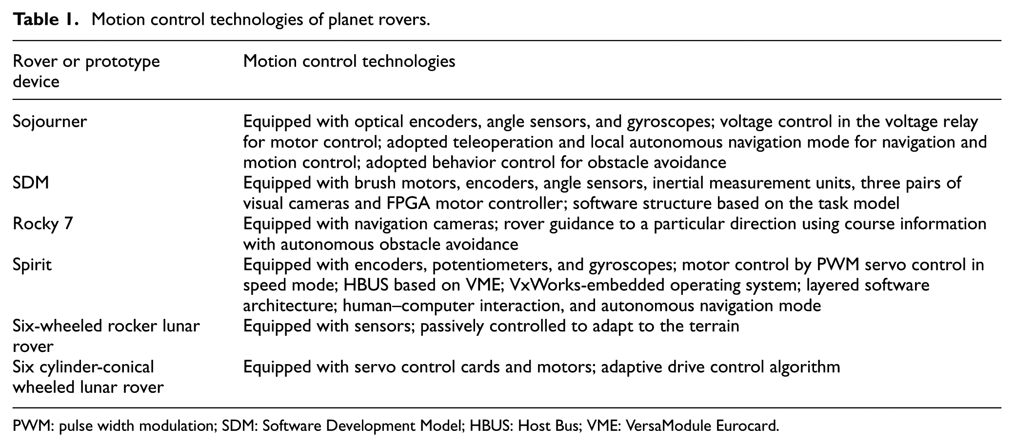
PWM: pulse width modulation; SDM: Software Development Model; HBUS: Host Bus; VME: VersaModule Eurocard.

It can be observed from Table 1 that not only the motion control algorithm but also fully equipped sensors are necessary to control the lunar rover. These sensors provide effective information to the motion control algorithm.

The energy of the lunar rover is mainly provided by solar panels and energy storage devices. The on-board power source can only provide extremely limited energy because of launch space and weight. Power generated by the solar panels is also affected by several factors, such as the solar panel area, lunar rover working area, sunshine duration, and sun angle. Therefore, the instantaneous power and energy efficiency of the motion system are quite demanding. The useless power consumption of the lunar rover should be reduced as much as possible during lunar exploration.

At present, control methods of the six-wheeled rocker lunar rover primarily consist of setting the same driving parameters for each wheel. This type of control method ignores the multiple active driving characteristics of the lunar rover and causes parasitic power loss. Thus, optimization of the energy utilization for motion control programming has become a key technique for the development and verification of motion control subsystems. It is also a significant component for the design of a lunar rover.

Modeling of the six-wheeled rocker lunar rover

Basic assumptions

The structure of the six-wheeled rocker lunar rover is shown in Figure 1(e). Before the motion analysis, the model of the lunar rover is assumed and simplified according to its characteristics and previously published research content as follows:

1. The width of the wheels does not affect the motion of the lunar rover according to the size of the prototype. Additionally, the width of the rockers is relatively small. Thus, the widths of the rockers and wheels are ignored in the simplified model.

2. The six-wheeled rocker lunar rover can realize the function of a zero radius of gyration. Marching and steering are decoupled. Because this article is focused on the marching process, the steering mechanism is ignored.

3. The ground is assumed to be a rigid body. Deformation caused by compaction and bulldozing is ignored.

4. The contact surface between the wheel and the ground is simplified as the contact point because of assumption 3.

According to the above assumptions, the model of the six-wheeled rocker lunar rover is simplified as shown in Figure 2.

Figure 2.

Simplified model of the six-wheeled rocker lunar rover in the initial state.

Suspension parameters are shown in Table 2.

Table 2.

Suspension parameters.

Parameter	Definition
α 1	Angle between the rear wheel connecting rod and the vertical line
β 1	Angle between the main rocker arm and the vertical line
h 1	Height between the body hinge point and the driving wheel center
α 2	Angle between the mid wheel connecting rod and the vertical line
β 2	Angle between the deputy rocker arm and the vertical line
h 2	Height between the rocker hinge point and the driving wheel center
r	Driving wheel radius

Define $\lambda$ as the angle of the main rocker rotating around the body hinge point from the initial state (the state of the main rocker arm and the deputy rocker arm, while all driving wheel centers are the same height). Define $\gamma$ as the angle of the deputy rocker rotating around the rocker hinge point from the initial state. All of these angles use the counterclockwise direction as the positive direction.

In addition to the basic hypothesis of motion analysis, the interaction force between the ground and wheels is simplified to the reaction force and the driving force. The driving force is simplified to the result of the driving force coefficient multiplied by the reaction force using the existing model.^9–11 In this simplified model, differences between each driving force are covered, and driving forces of each wheel seldom reach the maximum at the same time. Therefore, driving forces of each wheel are independent in this article. Stress conditions of each part of the lunar rover and the coordinate system definition while driving on any rugged path are shown in Figures 3–5 according to the above assumptions.

Figure 3.

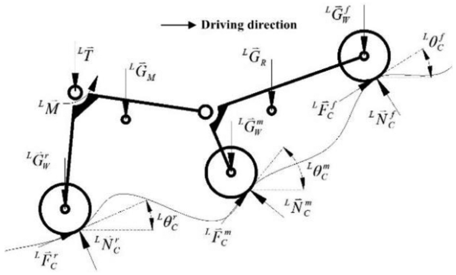
Quasi-static model of the left suspension of the six-wheeled rocker lunar rover.

Figure 4.

Quasi-static model of the right suspension of the six-wheeled rocker lunar rover.

Figure 5.

Lateral resistance of the six-wheeled rocker lunar rover.

Kinematic modeling of the lunar rover based on the theorem of projection velocities

Velocities of each part of the lunar rover while driving on the asymmetric rugged path are shown in Figure 6.

Figure 6.

Schematic diagram of the kinematics of the six-wheeled rocker lunar rover.

According to the analysis of parasitic power loss, slip and skid can be avoided and parasitic power loss can be eliminated if velocities of each point of the same component of the six-wheeled rocker lunar rover are in agreement with the velocity projection theorem.

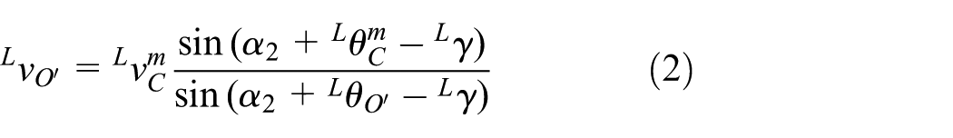
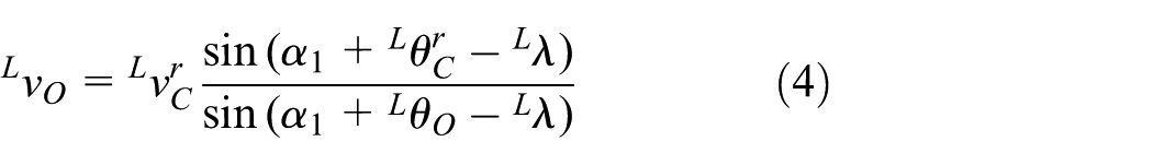
Then, velocities of the centers of the left front wheel and the left mid wheel of the left deputy rocker should meet the following equation

$$\mathrm{proj}({{}^L\stackrel{\rightharpoonup }{v}}_C^f,\overline{{{}^{L}W}^f{{}^{L}W}^m})=\mathrm{proj}({{}^L\stackrel{\rightharpoonup }{v}}_C^m,\overline{{{}^{L}W}^f{{}^{L}W}^m})$$

(1)

where ${{}^L\stackrel{\rightharpoonup }{v}}_C^f$ , ${{}^L\stackrel{\rightharpoonup }{v}}_C^m$ are the velocities of the centers of the left front wheel and the left mid wheel, respectively, ${{}^{L}v}_C^f=120\pi r{{}^{L}n}^r$ ; $\overline{{{}^{L}W}^f{{}^{L}W}^m}$ is the distance between the center of the left front wheel and the center of the left mid wheel. All similar variables have similar meanings in this article.

The instantaneous center of the velocity of the left deputy arm is determined by ${{}^L\stackrel{\rightharpoonup }{v}}_C^f$ and ${{}^L\stackrel{\rightharpoonup }{v}}_C^m$ . Then, the velocity of the left deputy rocker hinge point ${{}^L\stackrel{\rightharpoonup }{v}}_{O\prime }$ can be calculated by the following equation

$${{}^{L}v}_{O\prime }={{}^{L}v}_C^m\frac{\sin ({\alpha }_2+{{}^L\theta }_C^m-{}^L\gamma )}{\sin ({\alpha }_2+{{}^L\theta }_{O\prime }-{}^L\gamma )}$$

(2)

The left deputy rocker has the same velocity as the left deputy rocker hinge point because the hinge point turns without moving. The velocity of the left rear wheel and the left deputy rocker hinge point should meet the velocity projection theorem

$$\mathrm{proj}({{}^L\stackrel{\rightharpoonup }{v}}_C^r,\overline{{{}^{L}W}^r{{}^{L}O}^{\prime }})=\mathrm{proj}({{}^L\stackrel{\rightharpoonup }{v}}_{O\prime },\overline{{{}^{L}W}^r{{}^{L}O}^{\prime }})$$

(3)

where ${{}^L\stackrel{\rightharpoonup }{v}}_C^r$ is the velocity vector of the center of the left rear wheel.

The instantaneous center of the velocity of the left main rocker arm is determined by ${{}^L\stackrel{\rightharpoonup }{v}}_C^r$ and ${{}^L\stackrel{\rightharpoonup }{v}}_{O\prime }$ . Then, the velocity of the body hinge point ${{}^L\stackrel{\rightharpoonup }{v}}_O$ can be calculated by the following equation

$${{}^{L}v}_O={{}^{L}v}_C^r\frac{\sin ({\alpha }_1+{{}^L\theta }_C^r-{}^L\lambda )}{\sin ({\alpha }_1+{{}^L\theta }_O-{}^L\lambda )}$$

(4)

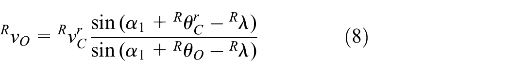
Similarly, the velocities of the wheel centers and hinge points of the right rocker arm can be calculated by the following equations

$$\mathrm{proj}({{}^R\stackrel{\rightharpoonup }{v}}_C^f,\overline{{{}^{R}W}^f{{}^{R}W}^m})=\mathrm{proj}({{}^R\stackrel{\rightharpoonup }{v}}_C^m,\overline{{{}^{R}W}^f{{}^{R}W}^m})$$

(5)

$${{}^R\stackrel{\rightharpoonup }{v}}_{O\prime }={{}^{R}v}_C^m\frac{\sin ({\alpha }_2+{{}^R\theta }_C^m-{}^R\gamma )}{\sin ({\alpha }_2+{{}^R\theta }_{O\prime }-{}^R\gamma )}$$

(6)

$$\mathrm{proj}({{}^R\stackrel{\rightharpoonup }{v}}_r^C,\overline{{{}^{R}W}^r{{}^{R}O}^{\prime }})=\mathrm{proj}({{}^R\stackrel{\rightharpoonup }{v}}_{O\prime },\overline{{{}^{R}W}^r{{}^{R}O}^{\prime }})$$

(7)

$${{}^{R}v}_O={{}^{R}v}_C^r\frac{\sin ({\alpha }_1+{{}^R\theta }_C^r-{}^R\lambda )}{\sin ({\alpha }_1+{{}^R\theta }_O-{}^R\lambda )}$$

(8)

The rocker–body hinge point of the main rocker arm has the same velocity as the body hinge point of the lunar rover body because the hinge point turns without moving. The velocity of the left body hinge point ${{}^L\stackrel{\rightharpoonup }{v}}_O$ and the velocity of the right body hinge point ${{}^R\stackrel{\rightharpoonup }{v}}_O$ should meet the velocity projection theorem

$$\mathrm{proj}({{}^L\stackrel{\rightharpoonup }{v}}_O,\overline{{}^{L}O{}^{R}O})=\mathrm{proj}({{}^R\stackrel{\rightharpoonup }{v}}_O,\overline{{}^{L}O{}^{R}O})$$

(9)

Thus, the kinematic model of the six-wheeled rocker lunar rover based on the velocity projection theorem is established. There is a proportional relationship between wheel speeds of each wheel. Slip and skid can be avoided as long as wheel speeds meet the proportional relationship of the velocity projection theorem. However, speed magnitudes cannot be determined by the velocity projection theorem. The speed of the driving wheels is limited by the maximum speed and driving power of the motor. Therefore, a mechanical analysis of the lunar rover is needed to determine the driving speed.

Quasi-static analysis of the six-wheeled rocker lunar rover

Quasi-static status is a type of critical status. In this status, forces are at a minimum in order to drive the lunar rover.

Equilibrium equations of each component

The equilibrium equation of the left suspension is

$$\begin{array}{c}{\stackrel{\rightharpoonup }{{}^{L}F}}_C^f+{\stackrel{\rightharpoonup }{{}^{L}F}}_C^m+{\stackrel{\rightharpoonup }{{}^{L}F}}_C^r+{\stackrel{\rightharpoonup }{{}^{L}N}}_C^f+{\stackrel{\rightharpoonup }{{}^{L}N}}_C^m+{\stackrel{\rightharpoonup }{{}^{L}N}}_C^r+{\stackrel{\rightharpoonup }{{}^{L}S}}_C^f+{\stackrel{\rightharpoonup }{{}^{L}S}}_C^m\hfill \\ +{\stackrel{\rightharpoonup }{{}^{L}S}}_C^r+{\stackrel{\rightharpoonup }{{}^{L}G}}_W^f+{\stackrel{\rightharpoonup }{{}^{L}G}}_W^m+{\stackrel{\rightharpoonup }{{}^{L}G}}_W^r+{{}^L\stackrel{\rightharpoonup }{G}}_M+{{}^L\stackrel{\rightharpoonup }{G}}_R+{}^L\stackrel{\rightharpoonup }{T}=0\hfill \end{array}$$

(10)

The equilibrium equation of the right suspension is

$$\begin{array}{c}{\stackrel{\rightharpoonup }{{}^{R}F}}_C^f+{\stackrel{\rightharpoonup }{{}^{R}F}}_C^m+{\stackrel{\rightharpoonup }{{}^{R}F}}_C^r+{\stackrel{\rightharpoonup }{{}^{R}N}}_C^f+{\stackrel{\rightharpoonup }{{}^{R}N}}_C^m+{\stackrel{\rightharpoonup }{{}^{R}N}}_C^r+{\stackrel{\rightharpoonup }{{}^{R}S}}_C^f+{\stackrel{\rightharpoonup }{{}^{R}S}}_C^m\hfill \\ +{\stackrel{\rightharpoonup }{{}^{R}S}}_C^r+{\stackrel{\rightharpoonup }{{}^{R}G}}_W^f+{\stackrel{\rightharpoonup }{{}^{R}G}}_W^m+{\stackrel{\rightharpoonup }{{}^{R}G}}_W^r+{{}^R\stackrel{\rightharpoonup }{G}}_M+{{}^R\stackrel{\rightharpoonup }{G}}_R+{}^R\stackrel{\rightharpoonup }{T}=0\hfill \end{array}$$

(11)

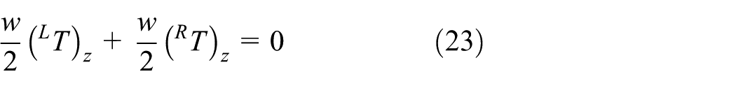
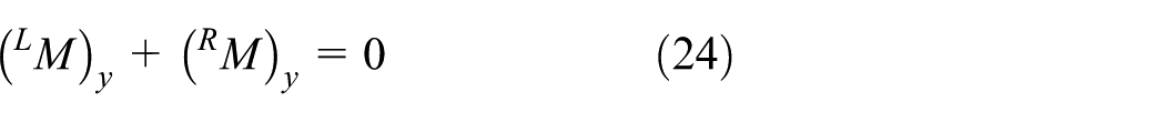
The equilibrium equation of the lunar rover body is

$${}^L\stackrel{\rightharpoonup }{T}+{}^R\stackrel{\rightharpoonup }{T}+{\stackrel{\rightharpoonup }{G}}_B=0$$

(12)

Torque equilibrium equations of each component

The torque equilibrium equation of the left deputy rocker arm is

$$\begin{array}{c}\overrightarrow{{{}^{L}O}^{\prime }{{}^{L}C}^f}\times ({\stackrel{\rightharpoonup }{{}^{L}F}}_C^f+{\stackrel{\rightharpoonup }{{}^{L}N}}_C^f+{\stackrel{\rightharpoonup }{{}^{L}S}}_C^f)\hfill \\ +\overrightarrow{{{}^{L}O}^{\prime }{{}^{L}W}^f}\times {\stackrel{\rightharpoonup }{{}^{L}G}}_W^f\hfill \\ +\overrightarrow{{{}^{L}O}^{\prime }{{}^{L}C}^m}\times ({\stackrel{\rightharpoonup }{{}^{L}F}}_C^m+{\stackrel{\rightharpoonup }{{}^{L}N}}_C^m+{\stackrel{\rightharpoonup }{{}^{L}S}}_C^m)\hfill \\ +\overrightarrow{{{}^{L}O}^{\prime }{{}^{L}W}^m}\times {\stackrel{\rightharpoonup }{{}^{L}G}}_W^m+\overrightarrow{{{}^{L}O}^{\prime }{}^{L}R}\times {{}^L\stackrel{\rightharpoonup }{G}}_R=0\hfill \end{array}$$

(13)

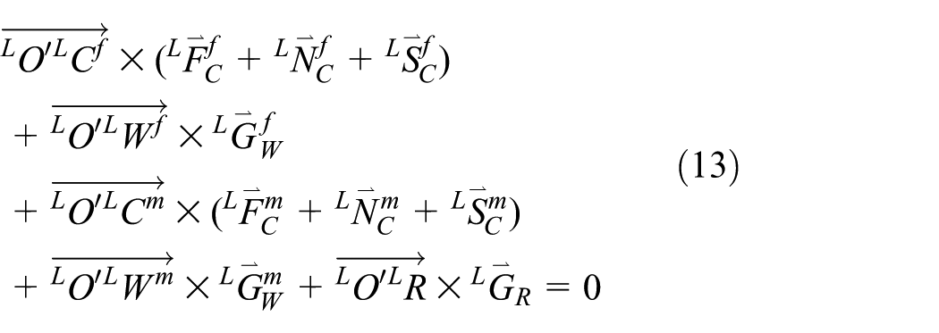
The torque equilibrium equation of the left main rocker arm is

$$\begin{array}{c}\overrightarrow{{{}^{L}O}^{\prime }{{}^{L}C}^r}\times ({\stackrel{\rightharpoonup }{{}^{L}F}}_C^r+{\stackrel{\rightharpoonup }{{}^{L}N}}_C^r+{\stackrel{\rightharpoonup }{{}^{L}S}}_C^r)\hfill \\ +\overrightarrow{{{}^{L}O}^{\prime }{{}^{L}W}^r}\times {\stackrel{\rightharpoonup }{{}^{L}G}}_W^r\hfill \\ +\overrightarrow{{{}^{L}O}^{\prime }{}^{L}M}\times {{}^L\stackrel{\rightharpoonup }{G}}_M\hfill \\ +\overrightarrow{{{}^{L}O}^{\prime }{}^{L}O\times }{}^L\stackrel{\rightharpoonup }{T}+{}^L\stackrel{\rightharpoonup }{M}=0\hfill \end{array}$$

(14)

The torque equilibrium equation of the right deputy rocker arm is

$$\begin{array}{c}\overrightarrow{{{}^{R}O}^{\prime }{{}^{R}C}^f}\times ({\stackrel{\rightharpoonup }{{}^{R}F}}_C^f+{\stackrel{\rightharpoonup }{{}^{R}N}}_C^f+{\stackrel{\rightharpoonup }{{}^{L}S}}_C^f)\hfill \\ +\overrightarrow{{{}^{R}O}^{\prime }{{}^{R}W}^f}\times {\stackrel{\rightharpoonup }{{}^{R}G}}_W^f\hfill \\ +\overrightarrow{{{}^{R}O}^{\prime }{{}^{R}C}^m}\times ({\stackrel{\rightharpoonup }{{}^{R}F}}_C^m+{\stackrel{\rightharpoonup }{{}^{R}N}}_C^m+{\stackrel{\rightharpoonup }{{}^{L}S}}_C^m)\hfill \\ +\overrightarrow{{{}^{R}O}^{\prime }{{}^{R}W}^m}\times {\stackrel{\rightharpoonup }{{}^{R}G}}_W^m+\overrightarrow{{{}^{R}O}^{\prime }{}^{R}R}\times {{}^R\stackrel{\rightharpoonup }{G}}_R=0\hfill \end{array}$$

(15)

The torque equilibrium equation of the right main rocker arm is

$$\begin{array}{c}\overrightarrow{{{}^{R}O}^{\prime }{{}^{R}C}^r}\times ({\stackrel{\rightharpoonup }{{}^{R}F}}_C^r+{\stackrel{\rightharpoonup }{{}^{R}N}}_C^r+{\stackrel{\rightharpoonup }{{}^{L}S}}_C^r)\hfill \\ +\overrightarrow{{{}^{R}O}^{\prime }{{}^{R}W}^r}\times {\stackrel{\rightharpoonup }{{}^{R}G}}_W^r\hfill \\ +\overrightarrow{{{}^{R}O}^{\prime }{}^{R}M}\times {{}^L\stackrel{\rightharpoonup }{G}}_R\hfill \\ +\overrightarrow{{{}^{R}O}^{\prime }{}^{R}O}\times {}^R\stackrel{\rightharpoonup }{T}+{}^R\stackrel{\rightharpoonup }{M}=0\hfill \end{array}$$

(16)

The torque equilibrium equation of the center of gravity of the rover body is

$$\overrightarrow{G{}^{L}O}\times {}^L\stackrel{\rightharpoonup }{T}+\overrightarrow{G{}^{R}O}\times {}^R\stackrel{\rightharpoonup }{T}+{}^L\stackrel{\rightharpoonup }{M}+{}^R\stackrel{\rightharpoonup }{M}=0$$

(17)

Thus, the quasi-static model of the six-wheeled rocker lunar rover has been established. Motor coordination torque and driving speed of the lunar rover in any attitude angle can be solved if the quasi-static model is coupled with the kinematic model.

It can be concluded that the above model is indefinite. Therefore, in this article, energy consumption is treated as an objective function, and the quasi-static model and the kinematic model are treated as constraint conditions for motor coordination programming of the lunar rover.

Optimization modeling of coordinated motion control aimed at energy consumption

Modeling of coordinated motion control

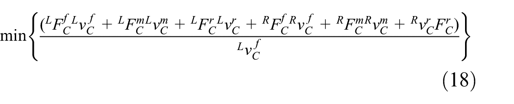
Objective function

The ultimate goal of coordinated motion control is saving energy. Therefore, the total energy consumption of six driving wheels can be calculated by the instantaneous power divided by the speed during the unit of time of the objective function. It is known from section “Basic assumptions” that the speeds of each wheel center have a proportional relationship with the speed of the barycenter of the lunar rover under coordinated motion control. Therefore, in the objective function, the instantaneous power of six wheels divided by the speed of the left front wheel is treated as an objective function of the coordinated motion control model instead of the instantaneous power of the six wheels divided by the speed of the barycenter

$$\begin{array}{c}min\left\{\frac{({{}^{L}F}_C^f{{}^{L}v}_C^f+{{}^{L}F}_C^m{{}^{L}v}_C^m+{{}^{L}F}_C^r{{}^{L}v}_C^r+{{}^{R}F}_C^f{{}^{R}v}_C^f+{{}^{R}F}_C^m{{}^{R}v}_C^m+{{}^{R}v}_C^r{F}_C^r)}{{{}^{L}v}_C^f}\right\}\hfill \end{array}$$

(18)

Constraint conditions

Constraint conditions of the quasi-static model

The vector equations of the quasi-static model are rewritten as scalar equations. Equations related to programming variables in the objective function are treated as constraint conditions.

According to the moment equilibrium of the left deputy rocker arm

$$\begin{array}{c}[{\left({{}^{L}O}^{\prime }{{}^{L}C}^f\right)}_z\cos {{}^L\theta }_C^f-{\left({{}^{L}O}^{\prime }{{}^{L}C}^f\right)}_x\sin {{}^L\theta }_C^f]{{}^{L}F}_C^f\hfill \\ -[{\left({{}^{L}O}^{\prime }{{}^{L}C}^f\right)}_z\sin {{}^L\theta }_C^f+{\left({{}^{L}O}^{\prime }{{}^{L}C}^f\right)}_x\cos {{}^L\theta }_C^f]{{}^{L}N}_C^f\hfill \\ +[{\left({{}^{L}O}^{\prime }{{}^{L}C}^m\right)}_z\cos {{}^L\theta }_C^m-{\left({{}^{L}O}^{\prime }{{}^{L}C}^m\right)}_x\sin {{}^L\theta }_C^m]{{}^{L}F}_C^m\hfill \\ -[{\left({{}^{L}O}^{\prime }{{}^{L}C}^m\right)}_z\sin {{}^L\theta }_C^m+{\left({{}^{L}O}^{\prime }{{}^{L}C}^m\right)}_x\cos {{}^L\theta }_C^m]{{}^{L}N}_C^m\hfill \\ -{\left({{}^{L}O}^{\prime }{{}^{L}W}^f\right)}_x{\left({{}^{L}G}_W^f\right)}_z-{\left({{}^{L}O}^{\prime }{}^{L}R\right)}_x{\left({{}^{L}G}_R\right)}_z\hfill \\ -{\left({{}^{L}O}^{\prime }{{}^{L}W}^m\right)}_x{\left({{}^{L}G}_W^m\right)}_z=0\hfill \end{array}$$

(19)

In the above equation, $({)}_x$ is the component vector of $()$ in the x-axis direction.

According to the moment equilibrium of the left main rocker arm

$$\begin{array}{c}[{\left({{}^{L}O}^{\prime }{{}^{L}C}^r\right)}_z\cos {{}^L\theta }_C^r-{\left({{}^{L}O}^{\prime }{{}^{L}C}^r\right)}_x\sin {{}^L\theta }_C^r]{{}^{L}F}_C^r\hfill \\ -[{\left({{}^{L}O}^{\prime }{{}^{L}C}^r\right)}_z\sin {{}^L\theta }_C^r+{\left({{}^{L}O}^{\prime }{{}^{L}C}^r\right)}_x\cos {{}^L\theta }_C^r]{{}^{L}N}_C^r\hfill \\ +{\left({{}^{L}O}^{\prime }{}^{L}O\right)}_z{\left({}^{L}T\right)}_x-{\left({{}^{L}O}^{\prime }{}^{L}O\right)}_x{\left({}^{L}T\right)}_z+{\left({}^{L}M\right)}_y\hfill \\ -{\left({{}^{L}O}^{\prime }{{}^{L}W}^r\right)}_x{\left({{}^{L}G}_W^r\right)}_z-{\left({{}^{L}O}^{\prime }{}^{L}M\right)}_x{\left({{}^{L}G}_M\right)}_z=0\hfill \end{array}$$

(20)

According to the moment equilibrium of the right deputy rocker arm

$$\begin{array}{c}[{\left({{}^{R}O}^{\prime }{{}^{R}C}^f\right)}_z\cos {{}^R\theta }_C^f-{\left({{}^{R}O}^{\prime }{{}^{R}C}^f\right)}_x\sin {{}^R\theta }_C^f]{{}^{R}F}_C^f\hfill \\ -[{\left({{}^{R}O}^{\prime }{{}^{R}C}^f\right)}_z\sin {{}^R\theta }_C^f+{\left({{}^{R}O}^{\prime }{{}^{R}C}^f\right)}_x\cos {{}^R\theta }_C^f]{{}^{R}N}_C^f\hfill \\ +[{\left({{}^{R}O}^{\prime }{{}^{R}C}^m\right)}_z\cos {{}^R\theta }_C^m-{\left({{}^{R}O}^{\prime }{{}^{R}C}^m\right)}_x\sin {{}^R\theta }_C^m]{{}^{R}F}_C^m\hfill \\ -[{\left({{}^{R}O}^{\prime }{{}^{R}C}^m\right)}_z\sin {{}^R\theta }_C^m+{\left({{}^{R}O}^{\prime }{{}^{R}C}^m\right)}_x\cos {{}^R\theta }_C^m]{{}^{R}N}_C^m\hfill \\ -{\left({{}^{R}O}^{\prime }{{}^{R}W}^f\right)}_x{\left({{}^{R}G}_W^f\right)}_z-{\left({{}^{R}O}^{\prime }{}^{R}R\right)}_x{\left({{}^{R}G}_R\right)}_z\hfill \\ -{\left({{}^{R}O}^{\prime }{{}^{R}W}^m\right)}_x{\left({{}^{R}G}_W^m\right)}_z=0\hfill \end{array}$$

(21)

According to the moment equilibrium of the right main rocker arm

$$\begin{array}{c}[{\left({{}^{R}O}^{\prime }{{}^{R}C}^r\right)}_z\cos {{}^R\theta }_C^r-{\left({{}^{R}O}^{\prime }{{}^{R}C}^r\right)}_x\sin {{}^R\theta }_C^r]{{}^{R}F}_C^r\hfill \\ -[{\left({{}^{R}O}^{\prime }{{}^{R}C}^r\right)}_z\sin {{}^R\theta }_C^r+{\left({{}^{R}O}^{\prime }{{}^{R}C}^r\right)}_x\cos {{}^R\theta }_C^r]{{}^{R}N}_C^r\hfill \\ +{\left({{}^{R}O}^{\prime }{}^{R}O\right)}_z{\left({}^{R}T\right)}_x-{\left({{}^{R}O}^{\prime }{}^{R}O\right)}_x{\left({}^{R}T\right)}_z+{\left({}^{R}M\right)}_y\hfill \\ -{\left({{}^{R}O}^{\prime }{{}^{R}W}^r\right)}_x{\left({{}^{R}G}_W^r\right)}_z-{\left({{}^{R}O}^{\prime }{}^{R}M\right)}_x{\left({{}^{R}G}_M\right)}_z=0\hfill \end{array}$$

(22)

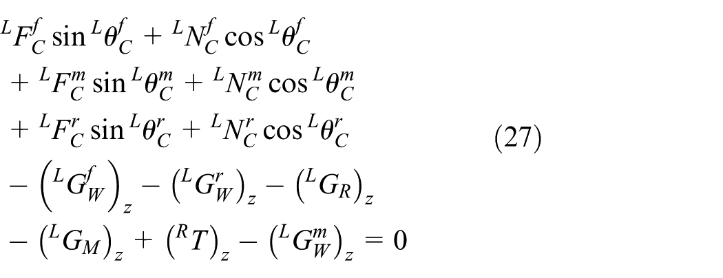
According to the moment equilibrium of the barycenter of the rover body

$$\frac{w}{2}{\left({}^{L}T\right)}_z+\frac{w}{2}{\left({}^{R}T\right)}_z=0$$

(23)

$${\left({}^{L}M\right)}_y+{\left({}^{R}M\right)}_y=0$$

(24)

$$-\frac{w}{2}{\left({}^{L}T\right)}_x-\frac{w}{2}{\left({}^{R}T\right)}_x=0$$

(25)

According to the force equilibrium of the left suspension

$$\begin{array}{c}{{}^{L}F}_C^f\cos {{}^L\theta }_C^f-{{}^{L}N}_C^f\sin {{}^L\theta }_C^f\hfill \\ -{{}^{L}N}_C^m\sin {{}^L\theta }_C^m+{{}^{L}F}_C^m\cos {{}^L\theta }_C^m\hfill \\ +{{}^{L}F}_C^r\cos {{}^L\theta }_C^r-{{}^{L}N}_C^r\sin {{}^L\theta }_C^r\hfill \\ +{\left({}^{L}T\right)}_x=0\hfill \end{array}$$

(26)

$$\begin{array}{c}{{}^{L}F}_C^f\sin {{}^L\theta }_C^f+{{}^{L}N}_C^f\cos {{}^L\theta }_C^f\hfill \\ +{{}^{L}F}_C^m\sin {{}^L\theta }_C^m+{{}^{L}N}_C^m\cos {{}^L\theta }_C^m\hfill \\ +{{}^{L}F}_C^r\sin {{}^L\theta }_C^r+{{}^{L}N}_C^r\cos {{}^L\theta }_C^r\hfill \\ -{\left({{}^{L}G}_W^f\right)}_z-{\left({{}^{L}G}_W^r\right)}_z-{\left({{}^{L}G}_R\right)}_z\hfill \\ -{\left({{}^{L}G}_M\right)}_z+{\left({}^{R}T\right)}_z-{\left({{}^{L}G}_W^m\right)}_z=0\hfill \end{array}$$

(27)

According to the force equilibrium of the right suspension

$$\begin{array}{c}{{}^{R}F}_C^f\cos {{}^R\theta }_C^f-{{}^{R}N}_C^f\sin {{}^R\theta }_C^f\hfill \\ -{{}^{R}N}_C^m\sin {{}^R\theta }_C^m+{{}^{R}F}_C^r\cos {{}^R\theta }_C^r\hfill \\ -{{}^{R}N}_C^r\sin {{}^R\theta }_C^r+{{}^{R}F}_C^m\cos {{}^R\theta }_C^m+\left({}^{R}T\right)=0\hfill \end{array}$$

(28)

$$\begin{array}{c}{{}^{R}F}_C^f\sin {{}^R\theta }_C^f+{{}^{R}N}_C^f\cos {{}^R\theta }_C^f+{{}^{R}F}_C^m\sin {{}^L\theta }_C^m\hfill \\ +{{}^{R}N}_C^m\cos {{}^R\theta }_C^m+{{}^{R}F}_C^r\sin {{}^R\theta }_C^r+{{}^{R}N}_C^r\cos {{}^R\theta }_C^r\hfill \\ -{\left({{}^{R}G}_W^f\right)}_z-{\left({{}^{R}G}_W^r\right)}_z-{\left({{}^{R}G}_R\right)}_z-{\left({{}^{R}G}_M\right)}_z\hfill \\ +{\left({}^{R}T\right)}_z-{\left({{}^{R}G}_W^m\right)}_z=0\hfill \end{array}$$

(29)

According to the force equilibrium of the rover body

$${\left({}^{L}T\right)}_x+{\left({}^{R}T\right)}_x=0$$

(30)

$${\left({}^{L}T\right)}_z+{\left({}^{R}T\right)}_z-{\left(G_B\right)}_z=0$$

(31)

Constraint conditions of the kinematic model

The vector equations of the kinematic model of the six-wheeled rocker lunar rover based on the velocity projection theorem are rewritten as scalar equations. Equations related to the programming variables in the objective function are selected and written as the velocity relationship between two points in the same component that are used as constraint conditions.

Taking the left front wheel and the left mid wheel of the left deputy rocker arm as objects

$${{}^{L}v}_C^f\cos ({{}^L\theta }_C^f-{}^L\gamma )={{}^{L}v}_C^m\cos ({{}^L\theta }_C^m-{}^L\gamma )$$

(32)

Taking the left mid wheel and the left rocker hinge point of the left deputy rocker arm as objects

$${{}^{L}v}_C^m\sin ({\alpha }_2+{{}^L\theta }_C^m-{}^L\gamma )={{}^{L}v}_{O\prime }\sin ({\alpha }_2+{{}^L\theta }_{O\prime }-{}^L\gamma )$$

(33)

Taking the left rear wheel and the left rocker hinge point of the left main rocker arm as objects

$${{}^{L}v}_C^r\cos ({{}^L\theta }_C^r-{}^L\xi -{}^L\lambda )={{}^{L}v}_{O\prime }\cos ({{}^L\theta }_{O\prime }-{}^L\xi -{}^L\lambda )$$

(34)

Taking the left rear wheel and the left body hinge point of the left main rocker arm as objects

$${{}^{L}v}_C^r\sin ({\alpha }_1+{{}^L\theta }_C^r-{}^L\lambda )={{}^{L}v}_O\sin ({\alpha }_1+{{}^L\theta }_O-{}^L\lambda )$$

(35)

Taking the right front wheel and the right mid wheel of the right deputy rocker arm as objects

$${{}^{R}v}_C^f\cos ({{}^R\theta }_C^f-{}^R\gamma )={{}^{R}v}_C^m\cos ({{}^R\theta }_C^m-{}^R\gamma )$$

(36)

Taking the right mid wheel and the right rocker hinge point of the right deputy rocker arm as objects

$${{}^{R}v}_C^m\sin ({\alpha }_2+{{}^R\theta }_C^m-{}^R\gamma )={{}^{R}v}_{O\prime }\sin ({\alpha }_2+{{}^R\theta }_{O\prime }-{}^R\gamma )$$

(37)

Taking the right rear wheel and the right rocker hinge point of the right main rocker arm as objects

$${{}^{R}v}_C^r\cos ({{}^R\theta }_C^r-{}^R\xi -{}^R\lambda )={{}^{R}v}_{O\prime }\cos ({{}^R\theta }_{O\prime }-{}^R\xi -{}^R\lambda )$$

(38)

Taking the right rear wheel and the right body hinge point of the right main rocker arm as objects

$${{}^{R}v}_C^r\sin ({\alpha }_1+{{}^R\theta }_C^r-{}^R\lambda )={{}^{R}v}_O\sin ({\alpha }_1+{{}^R\theta }_O-{}^R\lambda )$$

(39)

Taking the left body hinge point and the right body hinge point as objects

$${{}^{L}v}_O={{}^{R}v}_O=v_O$$

(40)

In addition to the kinematic and quasi-static constraint conditions, other constraint conditions should be taken into account to limit the drive torque and the drive speed.

Constraint conditions of motor-rated power

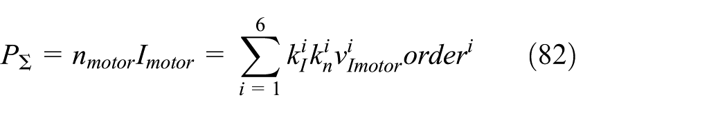
To give full play to the motor driving ability, at least one of these motors should reach the rated power, while all of the motors do not exceed the rated power. Thus

$$\begin{array}{c}max\{{{}^{L}F}_C^f{{}^{L}v}_C^f,{{}^{L}F}_C^m{{}^{L}v}_C^m,{{}^{L}F}_C^r{{}^{L}v}_C^r,\hfill \\ {{}^{R}F}_C^f{{}^{R}v}_C^f,{{}^{R}F}_C^m{{}^{R}v}_C^m,{{}^{R}F}_C^r{{}^{R}v}_C^r\}=P_0\hfill \end{array}$$

(41)

where $P_0$ is the rated power of the motors.

Constraint conditions of the maximum driving force of the motors

The maximum driving force of the motors should be larger than the required driving force of each wheel. Thus

$${{}^{i}F}_C^j<F_{max}(i=R,L;j=f,m,r)$$

(42)

where $F_{max}$ is the maximum driving force of motors

Constraint conditions of slipping

The required driving force of each wheel should be no larger than the driving force provided by the ground. Thus

$${{}^{i}F}_C^j-u{{}^{i}N}_C^j\le 0(i=R,L;j=f,m,r)$$

(43)

where u is the driving force coefficient of the ground.

Programming variables of the coordinated motion programming model

Mechanic and kinematic variables of the coordinated motion programming model are set to be programming variables. To facilitate systemizing these variables, they are set as follows

$$\begin{array}{c}{{}^{L}F}_C^f,{{}^{L}F}_C^m,{{}^{L}F}_C^r,{{}^{R}F}_C^f,{{}^{R}F}_C^m,{{}^{R}F}_C^r\hfill \\ =x_1,x_2,x_3,x_4,x_5,x_6\hfill \\ {{}^{L}v}_C^f,{{}^{L}v}_C^m,{{}^{L}v}_C^r,{{}^{R}v}_C^f,{{}^{R}v}_C^m,{{}^{R}v}_C^r\hfill \\ =x_7,x_8,x_9,x_{10},x_{11},x_{12}\hfill \\ {{}^{L}N}_C^f,{{}^{L}N}_C^m,{{}^{L}N}_C^r,{{}^{R}N}_C^f,{{}^{R}N}_C^m,{{}^{R}N}_C^r\hfill \\ =x_{13},x_{14},x_{15},x_{16},x_{17},x_{18}\hfill \\ {\left({}^{L}T\right)}_x,{\left({}^{L}T\right)}_z,{\left({}^{R}T\right)}_x,{\left({}^{R}T\right)}_z,{\left({}^{L}M\right)}_y,{\left({}^{R}M\right)}_y\hfill \\ =x_{19},x_{20},x_{21},x_{22},x_{23},x_{24}\hfill \\ {{}^{L}v}_{O\prime },{{}^R\stackrel{\rightharpoonup }{v}}_{O\prime },{{}^{L}v}_O,{{}^{R}v}_O=x_{25},x_{26},x_{27},x_{28}\hfill \end{array}$$

Systemizing the coordinated motion programming model

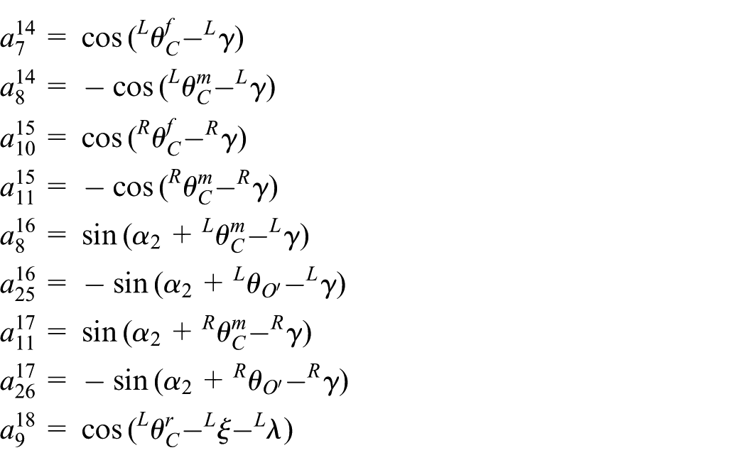
To solve the above equations, constraint conditions of the coordinated motion programming model are systemized. The systemized model is written as follows

$$\begin{array}{c}min\left\{\frac{(x_1{x}_7+x_2{x}_8+x_3{x}_9+x_4{x}_{10}+x_5{x}_{11}+x_6{x}_{12})}{x_{28}}\right\}\hfill \\ \left(\frac{(-b\pm \sqrt{b^2-4\mathrm{ac}})}{2a}\right)\hfill \\ =min\left\{\frac{(T_7{x}_1{x}_{28}+T_8{x}_2{x}_{28}+T_9{x}_3{x}_{28}+T_{10}{x}_4{x}_{28}+T_{11}{x}_5{x}_{28}+T_{12}{x}_6{x}_{28})}{x_{28}}\right\}\hfill \\ =min\{(T_7{x}_1+T_8{x}_2+T_9{x}_3+T_{10}{x}_4+T_{11}{x}_5+T_{12}{x}_6)\}\hfill \end{array}$$

(44)

In the above model

$$\begin{array}{c}{T}_7=\frac{a_8^{14}{a}_{25}^{16}{a}_9^{18}{a}_{27}^{20}}{a_7^{14}{a}_8^{16}{a}_{25}^{18}{a}_9^{20}},T_8=\frac{a_{25}^{16}{a}_9^{18}{a}_{27}^{20}}{a_8^{16}{a}_{25}^{18}{a}_9^{20}}\hfill \\ T_9=-\frac{a_{27}^{20}}{a_9^{20}},T_{10}=\frac{a_{11}^{15}{a}_{26}^{17}{a}_{12}^{19}{a}_{28}^{21}}{a_{10}^{15}{a}_{11}^{17}{a}_{26}^{19}{a}_{12}^{21}}\hfill \\ T_{11}=-\frac{a_{26}^{17}{a}_{12}^{19}{a}_{28}^{21}}{a_{11}^{17}{a}_{26}^{19}{a}_{12}^{21}},T_{12}=-\frac{a_{28}^{21}}{a_{12}^{21}}\hfill \end{array}$$

$$\begin{array}{l}{a}_7^{14}=\cos {(}^L{\theta }_C^f{-}^L\gamma )\\ a_8^{14}=-\cos {(}^L{\theta }_C^m{-}^L\gamma )\\ a_{10}^{15}=\cos {(}^R{\theta }_C^f{-}^R\gamma )\\ a_{11}^{15}=-\cos {(}^R{\theta }_C^m{-}^R\gamma )\\ a_8^{16}=\sin ({\alpha }_2{+}^L{\theta }_C^m{-}^L\gamma )\\ a_{25}^{16}=-\sin ({\alpha }_2{+}^L{\theta }_{O^{\prime }}{-}^L\gamma )\\ a_{11}^{17}=\sin ({\alpha }_2{+}^R{\theta }_C^m{-}^R\gamma )\\ a_{26}^{17}=-\sin ({\alpha }_2{+}^R{\theta }_{O^{\prime }}{-}^R\gamma )\\ a_9^{18}=\cos {(}^L{\theta }_C^r{-}^L\xi {-}^L\lambda )\end{array}$$

$$\begin{array}{c}{a}_{25}^{18}=-\cos {(}^L{\theta }_{O^{\prime }}{-}^L\xi {-}^L\lambda )\hfill \\ a_{12}^{19}=\cos {(}^R{\theta }_C^r{-}^R\xi {-}^R\lambda )\hfill \\ a_{26}^{19}=-\cos {(}^R{\theta }_{O\prime }{-}^R\xi {-}^R\lambda )\hfill \\ a_9^{20}=\sin ({\alpha }_1{+}^L{\theta }_C^r{-}^L\lambda )\hfill \\ a_{27}^{20}=-\sin ({\alpha }_1{+}^L{\theta }_O{-}^L\lambda )\hfill \\ a_{12}^{21}=\sin ({\alpha }_1{+}^R{\theta }_C^r{-}^R\lambda )\hfill \\ a_{28}^{21}=\sin ({\alpha }_1{+}^R{\theta }_C{-}^R\lambda )\hfill \end{array}$$

Calculation of the coordinated motion programming model

Common methods for calculating the programming model include a software solution, the control table method, and an analytical solution. A software solution and the control table method are not ideal methods because the real-time performance and solution accuracy are relatively poor. If the analytical solution of the programming model can be calculated and set as the control basis, the optimal solution for coordinated motion control can be directly calculated. Much numerical calculation can be avoided through this method, so that the calculation efficiency can be improved. Thus, the analytical solution is adopted as the method for calculating the programming model in this article.

The systemizing process is quite complicated, as there are a large number of programming variables and constraint conditions. One common method is substituting systemized results into the objective function, transforming constrained programming into unconstrained programming and finally calculating the optimal solution by solving the gradient of the objective function. Thus, the objective function becomes complex, and calculating the extremum of the function is difficult. In this article, the Kuhn–Tucker condition is used for calculations.

Introduction of the Kuhn–Tucker condition

The Kuhn–Tucker condition is an important theorem of constrained optimization issues. ¹² In the issue

$$\begin{array}{c}minf(x)\hfill \\ s.t.s_i(x)\ge 0,i=1,2,\dots ,m\hfill \\ h_j(x)=0,j=1,2,\dots ,l\hfill \end{array}$$

1. x* is the local optimal solution;

2. $I=\{i|s_i(x^{*})=0,i=1,2,\dots ,m\}$ ;

3. $f(x),s_1(x),\dots ,s_m(x),h_1(x),\dots ,h_l(x)$ are differentiable at the x* point;

4. $\nabla s_i(x^{*})$ are linearly independent with $\nabla h_1(x^{*}),\dots ,\nabla h_l(x^{*})$ , $i\in I$ .

Therefore, ${\tau }_1,\dots ,{\tau }_m;{\lambda }_1,\dots ,{\lambda }_l$ exist, so that

$$\begin{array}{c}\nabla f(x)-\sum _{i=1}^m{\tau }_i\nabla s_i(x^{*})-\sum _{j=1}^l{\lambda }_j\nabla h_j(x^{*})=0\hfill \\ {\tau }_i{s}_i(x^{*})=0,i=1,2,\dots ,m\hfill \\ {\tau }_i\ge 0,i=1,2,\dots ,m\hfill \end{array}$$

Calculation of the coordinated motion programming model based on the Kuhn–Tucker condition

According to the Kuhn–Tucker condition

$$\begin{array}{c}\nabla f(x)-\sum _{i=1}^m{\tau }_i\nabla s_i(x^{*})-\sum _{j=1}^l{\lambda }_j\nabla h_j(x^{*})=0\hfill \\ T_7-({\lambda }_1{m}_1^1+{\lambda }_5{m}_1^5+{\lambda }_6{m}_1^6)-(-{\tau }_{18}{T}_7{x}_{28}^{*})=0\hfill \end{array}$$

(45)

$$T_8-({\lambda }_1{m}_2^1+{\lambda }_5{m}_2^5+{\lambda }_6{m}_2^6)-(-{\tau }_{13}{T}_8{x}_{28}^{*})=0$$

(46)

$$T_9-({\lambda }_2{m}_3^2+{\lambda }_5{m}_3^5+{\lambda }_6{m}_3^6)-(-{\tau }_{14}{T}_9{x}_{28}^{*})=0$$

(47)

$$T_{10}-({\lambda }_3{m}_4^3+{\lambda }_7{m}_4^7+{\lambda }_8{m}_4^8)-(-{\tau }_{15}{T}_{10}{x}_{28}^{*})=0$$

(48)

$$T_{11}-({\lambda }_3{m}_5^3+{\lambda }_7{m}_5^7+{\lambda }_8{m}_5^8)-(-{\tau }_{16}{T}_{11}{x}_{28}^{*})=0$$

(49)

$$T_{12}-({\lambda }_4{m}_6^4+{\lambda }_7{m}_6^7+{\lambda }_8{m}_6^8)-(-{\tau }_{17}{T}_{12}{x}_{28}^{*})=0$$

(50)

$$-({\lambda }_1{m}_{13}^1+{\lambda }_5{m}_{13}^5+{\lambda }_6{m}_{13}^6)=0$$

(51)

$$-({\lambda }_1{m}_{14}^1+{\lambda }_5{m}_{14}^5+{\lambda }_6{m}_{14}^6)=0$$

(52)

$$-({\lambda }_2{m}_{15}^2+{\lambda }_5{m}_{15}^5+{\lambda }_6{m}_{15}^6)=0$$

(53)

$$-({\lambda }_3{m}_{16}^3+{\lambda }_7{m}_{16}^7+{\lambda }_8{m}_{16}^8)=0$$

(54)

$$-({\lambda }_4{m}_{18}^4+{\lambda }_7{m}_{18}^7+{\lambda }_8{m}_{18}^8)=0$$

(55)

$$-({\lambda }_3{m}_{17}^3+{\lambda }_7{m}_{17}^7+{\lambda }_8{m}_{17}^8)=0$$

(56)

$$-(-{\lambda }_2+{\lambda }_4)=0$$

(57)

$$-(-{\tau }_{13}{T}_8-{\tau }_{14}{T}_9-{\tau }_{15}{T}_{10}-{\tau }_{16}{T}_{11}-{\tau }_{17}{T}_{12}-{\tau }_{18}{T}_7)=0$$

(58)

In the above equations

$$\begin{array}{l}{m}_1^1={\left({}^L{O}^{\prime }{{}^{L}C}^f\right)}_z\cos {{}^L\theta }_C^f-{\left({}^L{O}^{\prime }{{}^{L}C}^f\right)}_x\sin {{}^L\theta }_C^f\\ m_2^1={\left({}^L{O}^{\prime }{{}^{L}C}^m\right)}_z\cos {{}^L\theta }_C^m-{\left({}^L{O}^{\prime }{{}^{L}C}^m\right)}_x\sin {{}^L\theta }_C^m\\ m_{13}^1=-{\left({}^L{O}^{\prime }{{}^{L}C}^f\right)}_x\cos {{}^L\theta }_C^f-{\left({}^L{O}^{\prime }{{}^{L}C}^f\right)}_z\sin {{}^L\theta }_C^f\\ m_{14}^1=-{\left({}^L{O}^{\prime }{{}^{L}C}^m\right)}_x\cos {{}^L\theta }_C^m-{\left({}^L{O}^{\prime }{{}^{L}C}^m\right)}_z\sin {{}^L\theta }_C^m\\ m_3^2={\left({}^L{O}^{\prime }{{}^{L}C}^r\right)}_z\cos {{}^L\theta }_C^r-{\left({}^L{O}^{\prime }{{}^{L}C}^r\right)}_x\sin {{}^L\theta }_C^r\\ m_{15}^2=-{\left({}^L{O}^{\prime }{{}^{L}C}^r\right)}_x\cos {{}^L\theta }_C^r-{\left({}^L{O}^{\prime }{{}^{L}C}^r\right)}_z\sin {{}^L\theta }_C^r\\ m_{24}^2=-1,m_{24}^4=1\\ m_4^3={\left({}^R{O}^{\prime }{{}^{R}C}^f\right)}_z\cos {{}^R\theta }_C^f-{\left({}^R{O}^{\prime }{{}^{R}C}^f\right)}_x\sin {{}^R\theta }_C^f\\ m_5^3={\left({}^R{O}^{\prime }{{}^{R}C}^m\right)}_z\cos {{}^R\theta }_C^m-{\left({}^R{O}^{\prime }{{}^{R}C}^m\right)}_x\sin {{}^R\theta }_C^m\\ m_{16}^3=-{\left({}^R{O}^{\prime }{{}^{R}C}^f\right)}_x\cos {{}^R\theta }_C^f-{\left({}^R{O}^{\prime }{{}^{R}C}^f\right)}_z\sin {{}^R\theta }_C^f\\ m_{17}^3=-{\left({}^R{O}^{\prime }{{}^{R}C}^m\right)}_x\cos {{}^R\theta }_C^m-{\left({}^R{O}^{\prime }{{}^{R}C}^m\right)}_z\sin {{}^R\theta }_C^m\end{array}$$

$$\begin{array}{c}{m}_6^4={\left({{}^{R}O}^{\prime }{{}^{R}C}^r\right)}_z\cos {{}^R\theta }_C^r-{\left({{}^{R}O}^{\prime }{{}^{R}C}^r\right)}_x\sin {{}^R\theta }_C^r\hfill \\ m_{18}^4=-{\left({{}^{R}O}^{\prime }{{}^{R}C}^r\right)}_x\cos {{}^R\theta }_C^r-{\left({{}^{R}O}^{\prime }{{}^{R}C}^r\right)}_z\sin {{}^R\theta }_C^r\hfill \\ m_1^5=\cos {{}^L\theta }_C^f,m_2^5=\cos {{}^L\theta }_C^m,m_3^5=\cos {{}^L\theta }_C^r\hfill \\ m_{13}^5=-\sin {{}^L\theta }_C^f,m_{14}^5=-\sin {{}^L\theta }_C^m,m_{15}^5=-\sin {{}^L\theta }_C^r\hfill \\ m_1^6=\sin {{}^L\theta }_C^f,m_2^6=\sin {{}^L\theta }_C^m,m_3^6=\sin {{}^L\theta }_C^r\hfill \\ m_{13}^6=\cos {{}^L\theta }_C^f,m_{14}^6=\cos {{}^L\theta }_C^m,m_{15}^6=\cos {{}^L\theta }_C^r\hfill \\ m_4^7=\cos {{}^R\theta }_C^f,m_5^7=\cos {{}^R\theta }_C^m,m_6^7=\cos {{}^R\theta }_C^r\hfill \\ m_{16}^7=-\sin {{}^R\theta }_C^f,m_{17}^7=-\sin {{}^R\theta }_C^m,m_{18}^7=-\sin {{}^R\theta }_C^r\hfill \\ m_4^8=\sin {{}^R\theta }_C^f,m_5^8=\sin {{}^R\theta }_C^m,m_6^8=\sin {{}^R\theta }_C^r\hfill \\ m_{16}^8=\cos {{}^R\theta }_C^f,m_{17}^8=\cos {{}^R\theta }_C^m,m_{18}^8=\cos {{}^R\theta }_C^r\hfill \end{array}$$

Because ${\tau }_i{s}_i(x^{*})=0$

$${\tau }_{13}(P_0-T_8{x}_2^{*}{x}_{28}^{*})=0$$

(59)

$${\tau }_{14}(P_0-T_9{x}_3^{*}{x}_{28}^{*})=0$$

(60)

$${\tau }_{15}(P_0-T_{10}{x}_4^{*}{x}_{28}^{*})=0$$

(61)

$${\tau }_{16}(P_0-T_{11}{x}_5^{*}{x}_{28}^{*})=0$$

(62)

$${\tau }_{17}(P_0-T_{12}{x}_6^{*}{x}_{28}^{*})=0$$

(63)

$${\tau }_{18}(P_0-T_7{x}_1^{*}{x}_{28}^{*})=0$$

(64)

Equations (45)–(50) are substituted into equation (58). Combined with equations (59)–(64), there are only eight unknown numbers ${\lambda }_1-{\lambda }_8$ in these eight equations.

If any of ${\tau }_{13}-{\tau }_{18}$ equals 0, the eight unknown numbers will be calculated from these nine independent equations. Therefore, these independent equations have no solution in this condition. Thus, all wheels working at full power $({\lambda }_1-{\lambda }_8\ne 0)$ is one condition for having solutions for the programming model. In this condition, the existence of solutions still needs to be discussed according to the mechanical constraint equations and the kinematic constraint conditions.

According to the kinematic constraint conditions, if all wheels work at full power, they should meet the following equation

$$T_7{x}_1^{*}=T_8{x}_2^{*}=T_9{x}_3^{*}=T_{10}{x}_4^{*}=T_{11}{x}_5^{*}=T_{12}{x}_6^{*}=P$$

(65)

where P is the defined value for systemizing.

Homogeneous linear equations of 13 unknown numbers are the results of systemizing. If ranks of the coefficient matrix and the augmented matrix are both 13, the equations have a unique solution. Solving the equations under the premise of having a unique solution

$$x_{15}^{*}=\frac{C_1^{15}{x}_1^{*}+C_2^{15}{x}_2^{*}+C_3^{15}{x}_3^{*}+C^{15}}{D^{15}}$$

(66)

In the above equation

$$\begin{array}{c}{C}_1^{15}=m_1^1(m_{13}^5{m}_{14}^6-m_{14}^5{m}_{13}^6)-m_{13}^1(m_1^5{m}_{14}^6-m_{14}^5{m}_1^6)\hfill \\ +m_{14}^1(m_1^5{m}_{13}^6-m_{13}^5{m}_1^6)\hfill \\ C_2^{15}=m_2^1(m_{13}^5{m}_{14}^6-m_{14}^5{m}_{13}^6)+m_{13}^1(m_{14}^5{m}_2^6-m_2^5{m}_{14}^6)\hfill \\ -m_{14}^1(m_{13}^5{m}_2^6+m_2^5{m}_{13}^6)\hfill \\ C_3^{15}=-m_{13}^1(m_3^5{m}_{14}^6-m_{14}^5{m}_3^6)\hfill \\ +m_{14}^1(m_3^5{m}_{13}^6-m_{13}^5{m}_3^6)\hfill \\ C^{15}=m_{14}^5(m_{13}^1{n}^6-m_{13}^6{n}^1)+m_{13}^5(m_{14}^6{n}^1-m_{14}^1{n}^6)\hfill \\ D^{15}=m_{13}^1{m}_{15}^5{m}_{14}^6-m_{14}^1{m}_{15}^5{m}_{13}^6-m_{13}^1{m}_{14}^5{m}_{15}^6\hfill \\ +m_{14}^1{m}_{13}^5{m}_{15}^6\hfill \\ x_{18}^{*}=\frac{C_4^{18}{x}_4^{*}+C_5^{18}{x}_5^{*}+C_6^{18}{x}_6^{*}+C^{18}}{D^{18}}\hfill \end{array}$$

(67)

In the above equation

$$\begin{array}{c}{C}_4^{18}=m_4^3(m_{16}^7{m}_{17}^8-m_{17}^7{m}_{16}^8)-m_{16}^3(m_4^7{m}_{17}^8-m_{17}^7{m}_4^8)\hfill \\ +m_{17}^3(m_4^7{m}_{16}^8-m_{16}^7{m}_4^8)\hfill \\ C_5^{18}=-m_5^3(m_{17}^7{m}_{16}^8-m_{16}^7{m}_{17}^8)-m_{16}^3(m_5^7{m}_{17}^8-m_{17}^7{m}_5^8)\hfill \\ +m_{17}^3(m_5^7{m}_{16}^8-m_{16}^7{m}_5^8)\hfill \\ C_6^{18}=-m_{16}^3(m_6^7{m}_{17}^8-m_{17}^7{m}_6^8)+m_{17}^3(m_6^7{m}_{16}^8-m_{16}^7{m}_6^8)\hfill \\ C^{18}=(m_{16}^7{m}_{17}^8-m_{17}^7{m}_{16}^8)(n^3+n^8)\hfill \\ D^{18}=m_{16}^3(m_{18}^7{m}_{17}^8-m_{17}^7{m}_{18}^8)-m_{17}^3(m_{18}^7{m}_{16}^8-m_{16}^7{m}_{17}^8)\hfill \\ x_{24}^{*}=\frac{m_3^2{x}_3+m_{15}^2{x}_{15}+n^2}{m_{24}^2}=\frac{m_6^4{x}_6+m_{18}^4{x}_{18}+n^4}{m_{24}^4}\hfill \end{array}$$

(68)

Substitute (66), (67), $x_3^{*}=P/T_9$ , and $x_6^{*}=P/T_{12}$ into equation (68)

$$P=\frac{\mathrm{FENZ}{I}_P}{\mathrm{FENM}{U}_P}$$

(69)

In the above equation

$$\begin{array}{c}\mathrm{FENZ}{I}_P=[m_{23}^2{m}_{18}^4{D}^{15}-m_{15}^2{m}_{24}^4{C}^{15}{D}^{18}\hfill \\ +(m_{24}^2{n}^4-m_{24}^4{n}^2)D^{15}{D}^{18}]T_7{T}_8{T}_9{T}_{10}{T}_{11}{T}_{12}\hfill \end{array}$$

(70)

$$\begin{array}{c}\multicolumn{1}{c}{\mathrm{FENM}{U}_P=m_3^2{m}_{24}^4{D}^{15}{D}^{18}{T}_7{T}_8{T}_{10}{T}_{11}{T}_{12}}\\ +m_{15}^2{m}_{24}^4{C}_1^{15}{D}^{18}{T}_8{T}_9{T}_{10}{T}_{11}{T}_{12}\hfill \\ +m_{15}^2{m}_{24}^4{C}_2^{15}{D}^{18}{T}_7{T}_9{T}_{10}{T}_{11}{T}_{12}\hfill \\ +m_{15}^2{m}_{24}^4{C}_3^{15}{D}^{18}{T}_7{T}_8{T}_{10}{T}_{11}{T}_{12}\hfill \\ -m_{24}^2{m}_6^4{D}^{15}{D}^{18}{T}_7{T}_8{T}_9{T}_{10}{T}_{11}\hfill \\ -m_{24}^2{m}_{18}^4{C}_4^{18}{D}^{15}{T}_7{T}_8{T}_9{T}_{11}{T}_{12}\hfill \\ -m_{24}^2{m}_{18}^4{C}_5^{18}{D}^{15}{T}_7{T}_8{T}_9{T}_{10}{T}_{12}\hfill \\ -m_{24}^2{m}_{18}^4{C}_6^{18}{D}^{15}{T}_7{T}_8{T}_9{T}_{10}{T}_{11}\hfill \end{array}$$

(71)

The optimal driving force of each wheel is shown as follows

$$x_1^{*}=\frac{P}{T_7},x_2^{*}=\frac{P}{T_8},x_3^{*}=\frac{P}{T_9},x_4^{*}=\frac{P}{T_{10}},x_5^{*}=\frac{P}{T_{11}},x_6^{*}=\frac{P}{T_{12}}$$

(72)

The optimal driving speed of each wheel is shown as follows

$$x_7^{*}=T_7,x_{28}^{*}=T_7\frac{P_0}{P}$$

(73)

$$x_8^{*}=T_8,x_{28}^{*}=T_8\frac{P_0}{P}$$

(74)

$$x_9^{*}=T_9,x_{28}^{*}=T_9\frac{P_0}{P}$$

(75)

$$x_{10}^{*}=T_{10},x_{28}^{*}=T_{10}\frac{P_0}{P}$$

(76)

$$x_{11}^{*}=T_{11},x_{28}^{*}=T_{11}\frac{P_0}{P}$$

(77)

$$x_{12}^{*}=T_{12},x_{28}^{*}=T_{12}\frac{P_0}{P}$$

(78)

Thus, the analytical solution of the optimal solution of the coordinated motion programming model has been calculated. The optimal solution is written as the optimal driving torque and optimal driving speed.

Simulation of the coordinated motion control model of the six-wheeled rocker lunar rover

Simulation modeling of the coordinated motion control model

Simulation of the lunar rover driving on a random asymmetric pavement based on ADAMS has been carried out to verify the validity of the coordinated motion control model. The simulation model is shown in Figure 7.

Figure 7.

Simulation model of the coordinated motion control.

The parameters of the prototype device in the simulation model are shown in Table 3. The emphasis of the simulation is the kinematic simulation; the control object is the speed of the driving wheel. Therefore, in the simulation, driving the model applies the motion function to the rover body rather than applying torque to the driving wheels. The driving force for the defined motion can be automatically calculated from the motion function. Thus, the effect of the control can be measured by measuring the driving force that is necessary for maintaining the motion.

Table 3.

Simulation model parameters.

Parameter/unit	α 1/°	β 1/°	h 1/mm	α 2/°	β 2/°	h 2/mm	r/mm
Value	45	45	500	45	45	250	100
Parameter/unit	GB/N	GM/N	GR/N	Gf/N	Gm/N	Gr/N	µ
Value	250	15	10	40	40	40	0.2

Results and analysis of the simulation

The model function of the coordinated motion control is edited in ADAMS. Attitude angles of the lunar rover are measured in ADAMS. These angles are input into the coordinated motion control model to calculate the coordinated motion control parameters and control driving of each model wheel. The required torque for maintaining the driving speed of each wheel is measured in the motion force function in ADAMS. Next, the simulation model is operated again, while the control parameters of each wheel are the same. Maintaining torque in this control condition is measured and compared with maintaining torque in the coordinated control condition. Curves for maintaining the torque of each wheel in these two simulations are shown in Figure 8.

Figure 8.

Maintaining torque of each wheel: (a) left front wheel, (b) left mid wheel, (c) left rear wheel, (d) right front wheel, (e) right mid wheel, and (f) right rear wheel.

From the integral curves, it is known that the sum of maintaining the torque in coordinated control is less than the sum of maintaining the torque at the same driving speed. In some cases, maintaining the torque of some wheel in coordinated control is larger than maintaining the torque at the same driving speed. When the driving parameters of each wheel are the same, some wheels are in the wheelspin condition, while some other wheels are in the sliding condition. The wheel in the sliding condition is pulled forward. Thus, maintaining the torque of the sliding wheel is less than maintaining the torque of the wheelspin wheel. The same driving parameters of each wheel can lead to an uneven distribution of driving force. However, all of these factors cannot affect the availability of the coordinated motion control model.

Experiments and analysis of the coordinated motion control model

To test the feasibility of the coordinated motion control model and verify the effectiveness of motion control, it is necessary to perform experiments.

Components of the prototype device

The prototype device consists of the hardware system and the software device. The hardware system consists of the six-wheeled rocker lunar rover, the upper PC (serial port expansion card PCI to serial port 2), the MCDC2805 AD/DA module, the MAXON ADS50/5 driver module, the sensor module (including AME-A001 swing angle sensors, AT-201-Sdoem attitude angle sensors, and motor current sensors), and the power module. The prototype device has the same parameters with the simulation model, which are shown in Table 3.

The software system is mainly responsible for reading the sensor data, controlling the calculation of the control strategy model, and transferring control instructions to the underlying driving system. According to the control process, the software system is composed of the control model algorithm program, the sensor data reading program, and the AD/DA control program. The prototype device is shown in Figure 9.

Figure 9.

Prototype device: (a) exterior of the prototype device and (b) hardware system of the prototype device.

Field experiments

The purpose of the coordinated control model is to eliminate or reduce parasitic power by controlling the driving speed of each wheel. Thus, two groups of contrasting experiments are carried out to validate the motion control effect:

1. Control stage of the same driving parameters. Attitude information of the lunar rover measured by the sensor system is input into the coordinated motion control algorithm. The driving speed of each wheel is calculated, and the minimum driving speed is given to each driving wheel to drive all wheels at the same speed. The electrical current of each motor is measured in order to compare the experimental results.

2. Control stage of the coordinated control model. The driving path of the first stage is repeated. Attitude information of the lunar rover measured by the sensor system is input into the coordinated motion control algorithm. The driving speed of each wheel is calculated and given to the corresponding wheel directly. The electrical current of each motor is measured in order to compare the experimental results.

A total of 10 random paths are chosen for these experiments. Because of the similarity and limited space, a random group of data is selected instead of all groups of data. The experimental process is shown in Figure 10.

Figure 10.

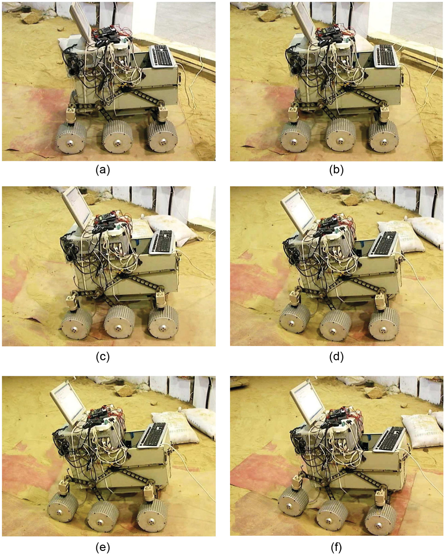
Experimental process of the prototype device in a random path.

According to the above analysis, state parameters (including the attitude angle and the speed of the rover body center) of the prototype device are input variables of the coordinated control model. State parameter curves of the prototype device in the selected experiment are shown in Figure 11. It can be observed from Figure 11 that motion control parameters change in real time because attitude angles change in real time.

Figure 11.

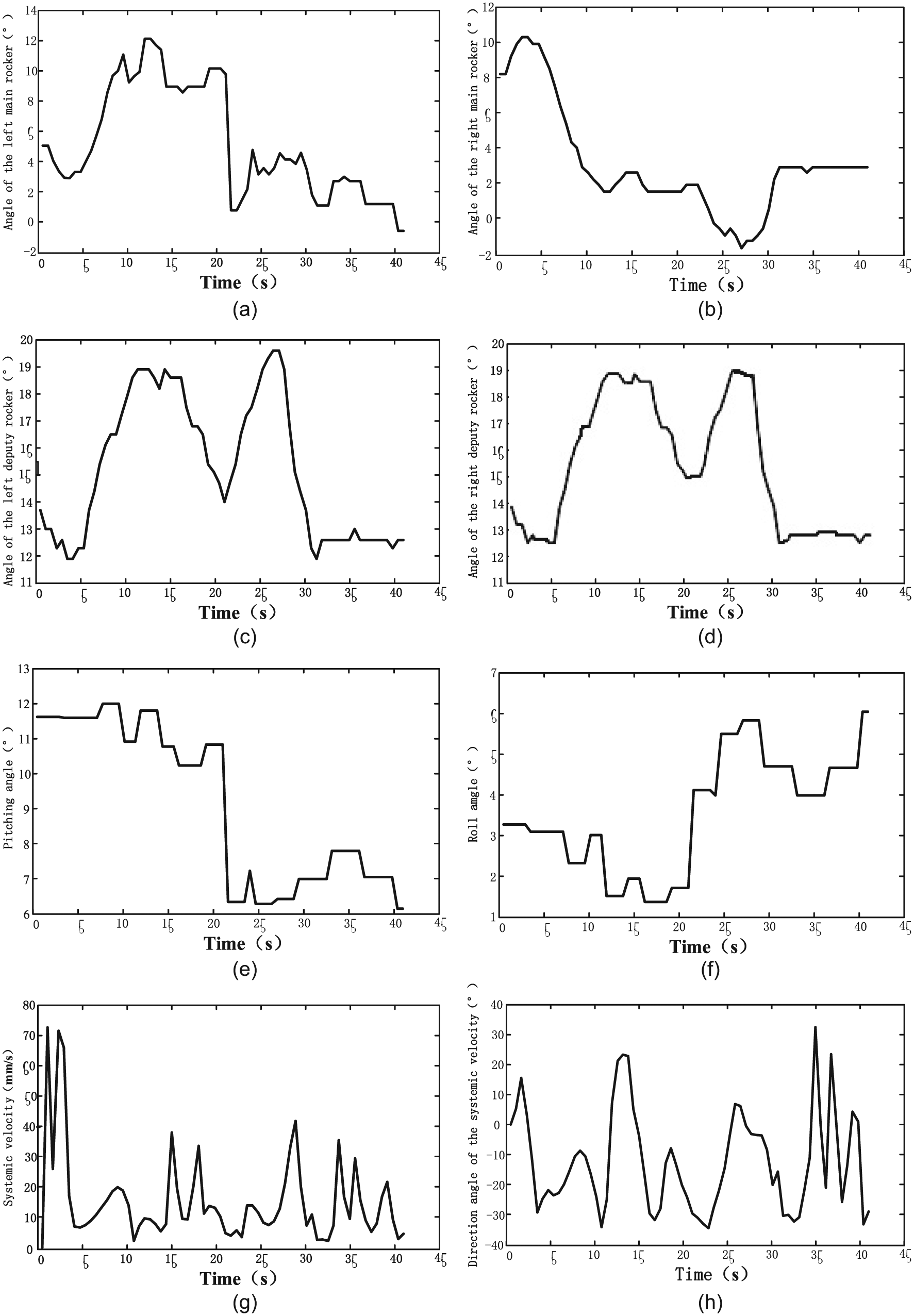
State parameters of the prototype device: (a) angle of the left main rocker, (b) angle of the right main rocker, (c) angle of the left deputy rocker, (d) angle of the right deputy rocker, (e) pitching angle, (f) roll angle, (g) systemic velocity, and (h) direction angle of the systemic velocity.

Attitude angles of the lunar rover are input into the coordinated motion control model to calculate coordinated motion control parameters of each wheel. Curves of the coordinated driving speed of each wheel are shown in Figure 12. It can be observed from Figure 12 that driving speeds of each wheel change in real time; these driving speeds are different as well. The variability of the driving speed is caused by the change in the attitude angle. Differences between driving speeds reflect the effectiveness of the coordinated motion control model.

Figure 12.

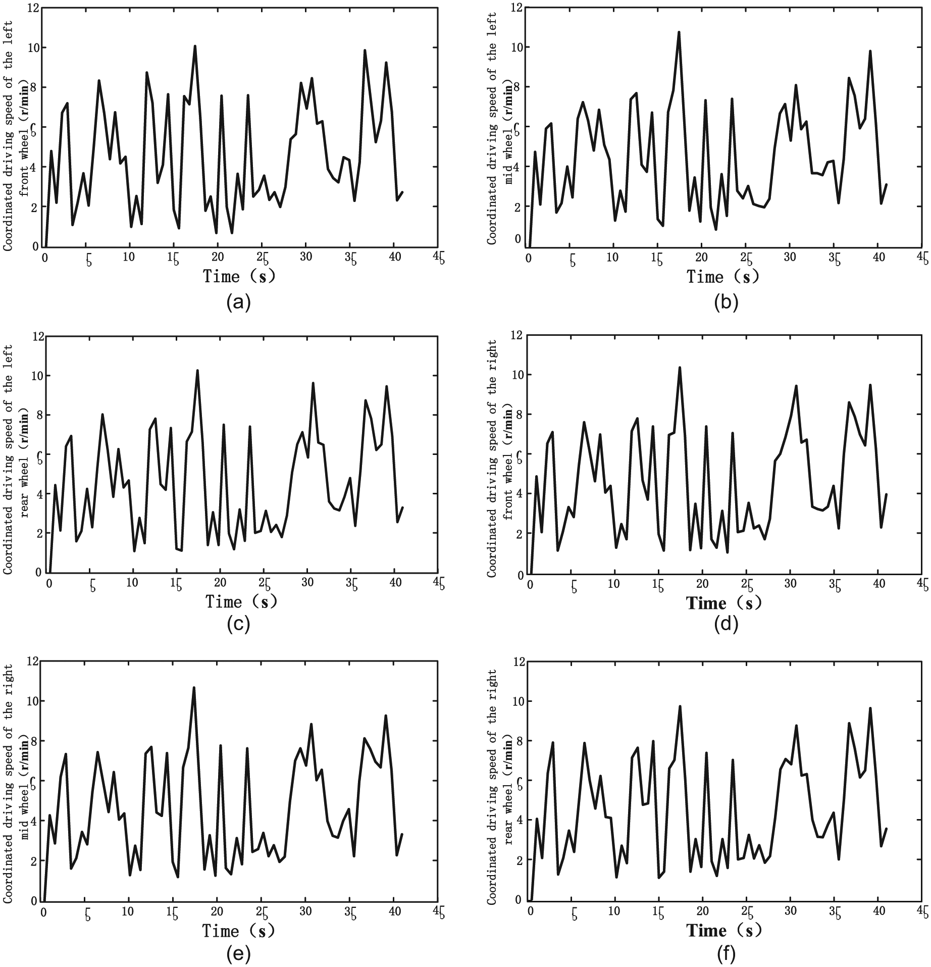
Coordinated driving speed of each wheel: (a) left front wheel, (b) left mid wheel, (c) left rear wheel, (d) right front wheel, (e) right mid wheel, and (f) right rear wheel.

Results and analysis of experiments

The output voltage of the driving motor current port is measured to assess the motor current indirectly. It can verify the effectiveness of the coordinated motion control model. Curves of output voltages of each driving motor current port are shown in Figure 13.

Figure 13.

Motor current of each wheel: (a) left front wheel, (b) left mid wheel, (c) left rear wheel, (d) right front wheel, (e) right mid wheel, and (f) right rear wheel.

It can be observed from Figure 13 that motor current changes in real time. It is affected by speed adjustment. However, the curves vary because of the frequent speed changes of the motors.

Motor current has a linear relationship with the output voltage of the driving motor current port

$$I_{\mathrm{motor}}=k_I\times V_{\mathrm{Imotor}}$$

(79)

where $I_{\mathrm{motor}}$ is the motor current; $k_I$ is the proportionality factor of current, according to the manual, $k_I=0.8(A/V)$ ; and $V_{\mathrm{Imotor}}$ is the output voltage of the driving motor current port.

Motor voltage has a linear relation with driving speed

$$V_{\mathrm{motor}}=k_V\times n_{\mathrm{motor}}$$

(80)

where $n_{\mathrm{motor}}$ is the driving speed; $k_V$ is the proportionality factor of voltage because the motor works in the speed mode, $k_V=10/n_{max}$ ; and $n_{max}$ is the maximum speed of the motor.

Therefore, the instantaneous power of the motor can be calculated by the following equation

$$P=V_{\mathrm{motor}}{I}_{\mathrm{motor}}=k_I{k}_n{V}_{\mathrm{Imotor}}{n}_{\mathrm{motor}}$$

(81)

where P is the instantaneous power of the motor.

The total power of the six driving wheels can be calculated by the following equation

$$P_{\Sigma }=n_{\mathrm{motor}}{I}_{\mathrm{motor}}=\sum _{i=1}^6{k}_I^i{k}_n^i{v}_{\mathrm{Imotor}}^i\mathrm{orde}{r}^i$$

(82)

where $P_{\Sigma }$ is the total power of six driving wheels.

The average power of each group of experiments is calculated from the total power function. Error caused by different driving speeds can be avoided because the average power is used as the experimental index. The average power of 10 groups of experiments is shown in Table 4.

Table 4.

Average power of coordinated motion control and same parameters control.

Path number	Average power (W)
	Same parameters control	Coordinated motion control	Energy saving rate (%)
1	48.58	47.61	2.0
2	54.06	51.85	4.1
3	50.48	49.00	5.4
4	52.09	50.37	3.3
5	59.74	57.64	3.5
6	57.04	56.70	0.6
7	50.62	50.26	0.7
8	55.56	53.78	3.2
9	55.74	55.12	1.1
10	46.51	47.61	4.8

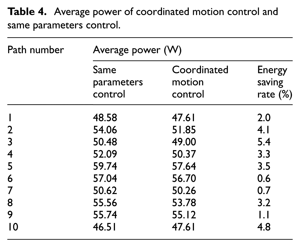
It can be observed from Table 4 that the coordinated motion control model has an effect of saving power. The energy savings rate is up to 5.4%, while the minimum energy savings rate is 0.6%.

Conclusion

In this article, a coordinated motion programming model of a six-wheeled rocker lunar rover based on the velocity projection theorem, quasi-static mechanical model, and motor-rated power is established to eliminate parasitic loss, reduce driving energy, and improve energy efficiency. The function of the model is the sum of the instantaneous power of the six wheels. Compared with other calculation methods, the analytical solution of the programming model based on the Kuhn–Tucker condition is chosen as the coordinated motion control model. To verify the effectiveness of the model, a series of experiments was performed. According to the comparison of experimental results of 10 random paths, the coordinated motion control model can effectively reduce driving energy. Considering the influence of the effective load distribution to the lunar rover, in further study, the deformation of the rocker arm will be considered in the coordinated motion control model to improve the control precision. The error correction link will be added to the Markov prediction control system to improve the prediction accuracy. The force model between the driving wheel and swampy lunar regolith will be added to the coordinated motion control system to improve the suitability of the coordinated motion control model for swampy lunar regolith.