Sage Journals: Discover world-class research

Abstract

Magnetorheological dampers have become prominent semi-active control devices for vibration mitigation of structures which are subjected to severe loads. However, the damping force cannot be controlled directly due to the inherent nonlinear characteristics of the magnetorheological dampers. Therefore, for fully exploiting the capabilities of the magnetorheological dampers, one of the challenging aspects is to develop an accurate inverse model which can appropriately predict the input voltage to control the damping force. In this article, a hybrid modeling strategy combining shuffled frog-leaping algorithm and adaptive-network-based fuzzy inference system is proposed to model the inverse dynamic characteristics of the magnetorheological dampers for improving the modeling accuracy. The shuffled frog-leaping algorithm is employed to optimize the premise parameters of the adaptive-network-based fuzzy inference system while the consequent parameters are tuned by a least square estimation method, here known as shuffled frog-leaping algorithm-based adaptive-network-based fuzzy inference system approach. To evaluate the effectiveness of the proposed approach, the inverse modeling results based on the shuffled frog-leaping algorithm-based adaptive-network-based fuzzy inference system approach are compared with those based on the adaptive-network-based fuzzy inference system and genetic algorithm–based adaptive-network-based fuzzy inference system approaches. Analysis of variance test is carried out to statistically compare the performance of the proposed methods and the results demonstrate that the shuffled frog-leaping algorithm-based adaptive-network-based fuzzy inference system strategy outperforms the other two methods in terms of modeling (training) accuracy and checking accuracy.

Keywords

Magnetorheological damper inverse model adaptive-network-based fuzzy inference system shuffled frog-leaping algorithm genetic algorithm

Introduction

Nowadays, it is challenging to find an effective means of protecting structures from dynamic hazards such as earthquakes and strong winds that may cause casualties and tremendous economic loss. Several control systems such as passive, active, and semi-active control systems have been developed to reduce structural vibration in the past two decades. Among these systems, the semi-active control system has become a hotspot recently, because it combines high reliability and low power requirement of the passive control system and significant adaptability and versatility of the active control system.¹

As one of the most promising semi-active control devices, the magnetorheological (MR) damper has received considerable interest.^2–7 It employs a type of smart material, that is, MR fluid to work reliably. The MR fluid has capability to change its viscosity from a viscous-fluid state to a semi-solid state instantaneously and reversibly by an applied magnetic field. Besides, it can generate large shear yield stress with low input voltage. Therefore, the MR damper exhibits many advantages such as large force capacity, high dynamic range, low power requirement, robustness, and mechanical simplicity.

To fully utilize the performance of the MR damper, it is desirable to control the damping force accurately generated by the MR damper. However, due to the multi-physics and intrinsic nonlinear dynamics of the MR damper, the damping force cannot be commanded directly. Only the input voltage of the MR damper can be directly controlled. Therefore, one of the important issues in the application of the MR damper is to develop an inverse model which can predict the input voltage to control the damping force accurately.

The techniques for developing the MR damper inverse model can be broadly classified into two categories: parametric and non-parametric techniques. The parametric inverse models of the MR damper are always derived from parametric forward models. Several parametric forward models described in terms of analogous mechanical elements have been developed.^8–13 Among them, the modified Bouc–Wen model is the most recognized one, which can accurately depict the nonlinear hysteresis of the MR damper over a wide range of operating conditions.⁹ However, its corresponding inverse model is difficult to obtain due to its nonlinearity and complexity. On the other hand, the non-parametric inverse modeling techniques for the MR damper have received considerable attention recently. These techniques mainly include fuzzy logic system,¹⁴ artificial neural networks (ANN),^3,15–17 and adaptive neuro-fuzzy inference system (ANFIS).^4,18

As for the fuzzy modeling technique, it has attractive advantages in handling uncertainties, high nonlinearities, and heuristic knowledge. However, the accuracy of the model highly depends on expert experience in selecting the large number of parameters that are used to define the membership functions (MFs) and the inference mechanisms. Therefore, fuzzy modeling the MR damper remains a challenging task. ANN can imitate the cognitive mechanism of the human brain to create an accurate model throughout learning and computation. However, it is challenging to design and analyze ANN in a transparent way because it is a black-box modeling framework.

ANFIS proposed by Jang¹⁹ adopts the combination of the fuzzy system and ANN to utilize the strengths of both, that is, the reasoning of fuzzy logic system and simple learning procedures and computational power of ANN. It has attracted the attention of many researchers and engineers and has been successfully applied in various fields.^20–24 Schurter and Roschke²⁵ initially adopted the ANFIS to model the forward dynamic behavior of the MR damper. Zeinali et al.²⁶ built the forward model with the ANFIS technique for two MR dampers of different strokes and investigated the effect of MF selection of the ANFIS on the model accuracy. Arsava and Kim⁵ successfully developed the MR damper forward model under a variety of impact loads on the basis of the ANFIS approach. It was experimentally demonstrated that the proposed ANFIS model performed better than other two parametric models. It can be pointed out here that researches dealing with the inverse dynamic behaviors of the MR damper with the ANFIS approach are relatively few. Nugroho et al.⁴ designed a MR damper inverse model using the ANFIS technique for the vibration control of a vehicle suspension. The results demonstrated that through the MR inverse model, the desired damping force can be accurately tracked by the predicted damping force.

Although ANFIS is a robust modeling technique, it needs an effective training algorithm to work successfully. In general, ANFIS employs a hybrid training algorithm combining gradient descent (GD) and least square estimation (LSE) methods to solve the parameter optimization.²⁷ The GD method may be good at recursive and exact computation, but it suffers from the problem of low convergence rate. Moreover, this algorithm gets stuck at local optima easily, thus definitely affecting the model accuracy.²⁷ Compared with the GD method, evolutionary algorithms (EAs) are more robust and efficient approaches for solving complex problems. For example, genetic algorithm (GA) is a kind of EAs which searches the optimal solution via simulating natural evolutionary process.²⁸ To overcome the drawbacks due to the GD method, some EAs and their variants have been introduced to determine the parameter setting of ANFIS such as GA,²⁹ particle swarm optimization (PSO)^30–32 and ant colony algorithm.³³

As a new member of EA family, shuffled frog-leaping algorithm (SFLA) was initially proposed and applied to the water distribution network by Eusuff and Lansey³⁴ in the year 2003. The SFLA conducts local search and global exploration for memetic evolution in the form of infection of ideas. The local search is similar to a PSO algorithm in concept. Compared with GA, SFLA is more simple and easy to be performed, because it neither has evolution operations such as crossover and mutation nor needs to adjust too many parameters. Actually, it combines the advantages of the genetic-based memetic algorithm and the social behavior-based PSO,³⁴ so it has attracted considerable attention in recent years.

Zhu and Zhang³⁵ proposed a modified SFLA to solve component pick-and-place sequencing optimization problem. The results demonstrated that both of the traditional SFLA and improved SFLA outperformed GA in terms of convergence accuracy. Gomez-Gonzalez et al.³⁶ used SFLA to estimate induction motor double-cage model parameters. The results revealed that SFLA surpassed PSO, GA, and a kind of modified Newton method. Perez et al.³⁷ employed SFLA to identify the equivalent circuit parameters of induction machines. The results indicated that SFLA performed better than PSO, GA, and differential evolution. Naghizadeh et al.³⁸ applied SFLA to determine parameters of Jiles–Atherton hysteresis model for representing magnetization in electrical steel sheets. The results showed that SFLA was faster and more accurate in comparison with other EAs including PSO, GA, differential evolution, and simulated annealing. Besides, in our previous study,³⁹ an intelligent control strategy integrating modified shuffled frog-leaping algorithm (MSFLA) and fuzzy logic controller (FLC) was proposed to mitigate the seismic vibration of structures installed with MR dampers. The MSFLA was used to adaptively optimize the FLC parameters. Then, the MSFLA-optimized FLC was employed to establish optimal relationship between seismic responses and command voltages of MR dampers. The results demonstrated that MSFLA performed better than GA in terms of convergence accuracy, and the MSFLA-optimized controller achieved better control of structural responses than the GA-optimized controller. Moreover, SFLA has also been successfully used to solve other challenging problems such as job shop scheduling,⁴⁰ compensation of atmospheric turbulence in optical communication systems,⁴¹ in-core fuel management optimization,⁴² and photovoltaic model identification.⁴³

In a word, SFLA has been proved to be a very promising and encouraging algorithm. In this study, motivated by the obvious advantages of SFLA, the algorithm is considered for an application in ANFIS parameter optimization, here known as SFLA-based ANFIS approach. To the best of our knowledge, this problem has not been studied before. Noted that although SFLA was also investigated in our previous study,³⁹ this study proposes a hybrid inverse modeling strategy for a MR damper, while Lin and Chen³⁹ proposed a hybrid control strategy for reducing the seismic responses of a structural building with MR dampers. In this study, for selecting the optimum parameters for SFLA, two-way analysis of variance (ANOVA) is employed to study the influences of the parameters for SFLA on the best solutions. To control the damping force of the MR damper more accurately, the SFLA-based ANFIS approach is proposed to develop the inverse model to predict input voltage of the MR damper. As far as we know, there has not been literature published about developing inverse model of the MR damper using the EA-optimized ANFIS strategy. Since GA is always a benchmark in EAs, for the sake of comparison, GA-based ANFIS strategy is also employed to model the inverse dynamic behaviors of the MR damper. The proposed hybrid strategy yields promising results as follows: (1) The SFLA-based ANFIS and GA-based ANFIS strategies significantly perform better than the ANFIS approach in terms of convergence accuracy and convergence speed. (2) The SFLA-based ANFIS strategy is superior to the GA-based ANFIS strategy in terms of training accuracy and checking accuracy. (3) The EA-optimized ANFIS with the fitness function F₂ yields better results than with fitness function F₁ in terms of convergence accuracy for both of training and checking data. (4) The target damping force can be most accurately tracked by the predicted damping force with the SFLA-based ANFIS strategy.

Description of the inverse MR damper model

The control of the MR damper is very important for all applications, but it is the input voltage, not the MR damping force that can be directly controlled. Therefore, an inverse model of the MR damper is required to build to predict the voltage for accurately controlling the damping force.

Inverse model of the MR damper and its application

Figure 1 illustrates the scheme of building and applying the MR damper inverse model. The modeling part in the figure describes how to develop the inverse model. At first, the modified Bouc–Wen model⁹ is chosen to build the MR damper forward model due to its high accuracy of characterizing the nonlinear dynamics. If displacement, velocity, and voltage (target voltage) are given, target damping force can be calculated through the forward model, which will be detailed in the following subsection. Then, the structure of the MR damper inverse model is designed with three inputs: displacement, velocity, and damping force. Finally, the inverse model is trained with the proposed SFLA-based ANFIS strategy until the smallest error between the predicted voltage (the output of the inverse model) and target voltage is attained, thus obtaining an optimal inverse model. The application part in the figure shows that on the basis of the predicted voltage, the forward model can output the predicted damping force to track the target damping force for vibration control.

Figure 1.

Development and application of the MR damper inverse model.

Forward model of MR damper

The forward dynamic behavior of the MR damper is portrayed by the modified Bouc–Wen model proposed by Spencer et al.⁹ The model is described as follows

f = α z + c_{0} (\overset{\cdot}{x} - \overset{\cdot}{y}) + k_{0} (x - y) + k_{1} (x - x_{0})

(1)

where the evolutionary variable y and z are governed by

\overset{\cdot}{y} = (\frac{1}{c_{0} + c_{1}}) {α z + c_{0} \overset{\cdot}{x} + k_{0} (x - y)}

(2)

and

\overset{\cdot}{z} = - γ | \overset{\cdot}{x} - \overset{\cdot}{y} | z | z |^{n - 1} - β (\overset{\cdot}{x} - \overset{\cdot}{y}) | z |^{n} + A (\overset{\cdot}{x} - \overset{\cdot}{y})

(3)

respectively. Here, f is the damping force; x and $\overset{\cdot}{x}$ are the displacement and velocity, respectively; k₁ is the accumulator stiffness; x₀ is the initial displacement of spring k₁ associated with the nominal damper force due to the accumulator; k₀ is the constant to control the stiffness at large velocities; γ, β, and A are hysteresis parameters for the yield element; α is evolutionary coefficient; c₀ and c₁ are viscous damping observed at large velocities and low velocities, respectively. α, c₀, and c₁ are calculated as follows

α = α (u) = α_{a} + α_{b} u

(4)

c_{1} = c_{1} (u) = c_{1 a} + c_{1 b} u

(5)

c_{0} = c_{0} (u) = c_{0 a} + c_{0 b} u

(6)

respectively, where u is given as the output of a first-order filter calculated as

\overset{\cdot}{u} = - η (u - v)

(7)

and v is the input voltage of the MR damper. A total of 14 model parameters of the MR damper are listed in the literature.⁹

Hybrid technique combining SFLA and ANFIS

An overview of SFLA

SFLA is a meta-heuristic optimization method which is inspired by the behavior of frogs when seeking for food.³⁴ The SFLA conducts searching using a population of frogs (solutions) which correspond to individuals in GA. In SFLA, each frog carries a single meme to represent its position which corresponds to a chromosome carried by the individual in GA. The frogs are allowed to communicate with each other to improve their memes and search for better location of food.

SFLA begins by randomly generating N frogs and sorting them according to the descending order of their fitness values. Next, the frogs are divided into m memeplexes, each containing n (m × n = N) frogs. The frogs are organized into the memeplexes in the way as follows: the frog ranked first is assigned into the first memeplex, the one ranked second into the second memeplex, the one ranked nth into the nth memeplex, the one ranked n + first into the first memeplex, the one ranked n + second into the second memeplex, and the sequence continues until all frogs are assigned.

In each memeplex, to avoid from falling in a local optimum, q frogs are selected to form a sub-memeplex with a strategy of triangular probability distribution.³⁴ The probability assigned to each frog is expressed as

p_{j} = \frac{2 (n + 1 - j)}{n (n + 1)} j = 1, 2, \dots, n

(8)

With this strategy, the frogs with larger fitness values (also called better frogs) have higher chances of being included in the sub-memeplex due to higher probabilities. Then, the worst and best frogs are searched from the sub-memeplex which are donated as X_W and X_B, respectively. In nature, the X_W tends to jump in the direction of the location of the X_B for having more food. However, due to imperfect perception, the X_W cannot locate exactly the position of the X_B. Moreover, it is possible that the X_W could jump over the X_B. Therefore, here a frog-leaping rule in Eusuff and Lansey³⁴ is adopted which is seen in equation (9)

X_{W}^{k + 1} (j) = X_{W}^{k} (j) + R (X_{B}^{k} (j) - X_{W}^{k} (j)) (j = 1, 2, \dots, l)

(9)

where k is the iteration number of the memeplex. The length of X_W, X_B, and R is l. R consists of l random numbers between 0 and 1. If the new frog is better than the previous frog, the previous frog will be replaced by the new one. Otherwise, the calculation in equation (9) is repeated in which the global best frog X_G substitutes the X_B. If still no improvement becomes possible, a new frog will be generated randomly to replace the X_W. After each iteration, the memeplex will be updated. If the fitness value of the new frog is larger than that of the global best frog X_G, then the X_G will be replaced with the new frog. Repeat this updating operation in each memeplex until the pre-defined iteration number k is satisfied.

After finishing the local deep-searching for all memeplexes, all of the frogs are shuffled into a new population and then reassigned into different memeplexes. The local searching and the shuffling processes alternate until the defined convergence criterion is satisfied. The flowchart of SFLA is illustrated in Figure 2.

Figure 2.

Flowchart of SFLA.

Architecture of ANFIS

The ANFIS model is a combination of a fuzzy system and a neural network. It can accurately predict the nonlinear behavior and generate input–output with high degree of accuracy. Figure 3 shows the structure of a two-input two-rule ANFIS which consists of the following five layers:¹⁹

Layer 1: every node i in this layer is a square node with an output defined by

\begin{matrix} O_{1, i} = μ_{A_{i}} (x_{1}), i = 1, 2 \\ O_{1, i} = μ_{B_{i - 2}} (x_{2}), i = 3, 4 \end{matrix}

(10)

where x₁ (or x₂) is the input to node i and A_i (or B_i_− 2) is the linguistic label (small, medium, large, etc.) associated with this node. µ_A (or µ_B) is a value of a MF which specifies the degree to which the input value belongs to a fuzzy set. Taking a generalized bell-shaped MF as an example, the MF value is expressed as follows

μ_{A_{i}} = \frac{1}{1 + {| (x_{1} - c_{i}) / a_{i} |}^{2 b_{i}}}

(11)

where a_i, b_i, and c_i are called MF parameters or premise parameters which represent the width, the slope at 0.5 membership grade and the central position of the MF, respectively.

Figure 3.

Architecture of a two-input-two-rule ANFIS.

Layer 2: every node in this layer is a circle node labeled π whose output is the product of all the incoming signals

O_{2, i} = w_{i} = μ_{A_{i}} (x_{1}) \times μ_{B_{i}} (x_{2}), i = 1, 2

(12)

Each output node represents the firing strength of a rule.

Layer 3: every node in this layer is a circle node labeled N. The ith node calculates the ratio of the ith rule’s firing strength to the sum of all rules’ firing strengths

O_{3, i} = {\bar{w}}_{i} = \frac{w_{i}}{w_{1} + w_{2}}, i = 1, 2

(13)

Outputs are called normalized firing strengths.

Layer 4: if the rules’ format for the network in Figure 3 is

Rule i: If x₁ is A and x₂ is B, then $f_{i} = p_{i} x_{1} + q_{i} x_{2} + r_{i}$ , where A and B are linguistic terms, then the output of this layer is calculated by

O_{4, i} = {\bar{w}}_{i} f_{i} = {\bar{w}}_{i} (p_{i} x_{1} + q_{i} x_{2} + r_{i}), i = 1, 2

(14)

where p_i, q_i, and r_i are called rule parameters or consequent parameters.

Layer 5: the single node in this layer is labeled Σ which computes the overall output as the summation of incoming signals

O_{5, i} = \sum_{i = 1}^{2} {\bar{w}}_{i} f_{i} = \frac{\sum_{i = 1}^{2} w_{i} f_{i}}{\sum_{i = 1}^{2} w_{i}}

(15)

SFLA-based ANFIS strategy for inverse modeling

The ANFIS structure shows that the nodes in Layers 1 and 4 are adaptive while the others are fixed. These adaptive nodes employ premise and consequent parameters which need to be optimized. The purpose of learning the ANFIS is to tune these parameters. Generally, the learning process of the ANFIS consists of two parts in each iteration. In the first part, the inputs are propagated forward and the consequent parameters are identified by the LSE method, while the premise parameters are assumed to be fixed. Observed from the above ANFIS architecture, based on the inputs, initial premise parameters and initial consequent parameters, the overall output y can be finally expressed as follows

\begin{matrix} y & = \sum_{i = 1}^{2} {\bar{w}}_{i} f_{i} = {\bar{w}}_{1} (p_{1} x_{1} + q_{1} x_{2} + r_{1}) + {\bar{w}}_{2} (p_{2} x_{1} + q_{2} x_{2} + r_{2}) \\ = ({\bar{w}}_{1} x_{1}) p_{1} + ({\bar{w}}_{1} x_{2}) q_{1} + {\bar{w}}_{1} r_{1} + ({\bar{w}}_{2} x_{1}) p_{2} + ({\bar{w}}_{2} x_{2}) q_{2} + {\bar{w}}_{2} r_{2} \\ = A θ \end{matrix}

(16)

where θ = {p₁, q₁, r₁, p₂, q₂, r₂} is a set of consequent parameters. If there are N sets of training data, the dimension of y, A, and θ are N × 1, N × 6 and 6 × 1, respectively. Here, 6 is the number of the consequent parameters. $\hat{θ}$ , also called estimated θ, is computed by the LSE method as shown in equation (17). Then, the output ŷ for the training data estimated by ANFIS is calculated according to equation (18)

\hat{θ} = (A^{T} A)^{- 1} A^{T} y

(17)

\hat{y} = A \hat{θ}

(18)

$\hat{θ}$ is calculated to minimize the root-mean-square error (RMSE) between the overall output y and the estimated output ŷ for the training data. Here, the RMSE value is calculated as

RMSE = 100 \times \sqrt{\frac{1}{N} \sum_{k = 1}^{N} {(y (k) - \hat{y} (k))}^{2}}

(19)

where N is the number of the training data sets. In the second part, the RMSE value is propagated backward while the estimated consequent parameter set is fixed, then the GD method is used to update the premise parameters. A general description of the GD algorithm is given by Haykin.²⁷ This hybrid learning procedure is iterated until the error is reduced to a desired goal or until a maximum number of training cycles is reached.

However, the GD method suffers from the problems of local minima and low convergence rate. Due to the superior performance of SFLA in solving complex problems, in this study, SFLA is introduced instead of GD to determine the premise parameters of ANFIS, while the LSE method is still used to solve the consequent parameters. The specific operation steps of the proposed SFLA-based ANFIS approach for developing the MR damper inverse model are detailed as follows:

1. Determining the ANFIS structure: the factors that determine the ANFIS structure should be pre-determined such as the number of inputs and outputs and the type and number of the MFs for each input.

2. Generating training data sets and checking data sets: the training data sets are used for training and determining the ANFIS parameters while the checking data sets are used for validating the generalization capability of the trained ANFIS.

3. Determining the parameter boundaries and encoding strategy: define the constraints of the premise and consequent parameters of the ANFIS according to the training data. Besides, real-number encoding strategy is employed. Taking the generalized bell-shaped MF as an example, the encoding of the premise parameters is shown as follows

a_{1} b_{1} c_{1} a_{2} b_{2} c_{2} \dots a_{i} b_{i} c_{i}

where i is the number of MFs for all inputs. The initial consequent parameters are generated randomly and also encoded with real numbers. Assuming that the number of inputs is 2 as shown in Figure 3, the consequent parameters are encoded as follows

p_{1} q_{1} r_{1} p_{2} q_{2} r_{2} \dots p_{j} q_{j} r_{j}

where j is the number of rules.

4. Building fitness function: fitness function is an effective function for measuring new solutions to distinguish the improved ones. It varies on different problems and purposes. In this study, two fitness functions are used in the proposed strategy. One fitness function is defined as follows

F_{1} = \frac{1}{1 + RMSE}

(20)

where the RMSE is the training error defined in equation (19). The smaller the RMSE is, the larger the fitness value is. The other fitness function is defined as follows

F_{2} = \frac{1}{1 + (w \times RMSE + (1 - w) \times RMS E_{chk})}

(21)

where w is a weighting coefficient reflecting the relative importance of RMSE and RMSE_chk. RMSE_chk is the error between the actual output y_chk and the predicted output ŷ_chk for the checking data sets which is calculated as

RMS E_{chk} = 100 \times \sqrt{\frac{1}{N} \sum_{k = 1}^{N} {(y_{chk} (k) - {\hat{y}}_{chk} (k))}^{2}}

(22)

where N is the number of the checking data sets. ŷ_chk can be calculated by reference to equation (18) through the checking data.

5. Initializing the SFLA: initialize the parameters such as population size, memeplex size, local iteration number, and global convergence criterion.

6. In the first cycle, generating initial solutions (frogs) and consequent parameters: based on the defined parameter boundaries and the SFLA’s setting parameters, randomly generate an initial population of solutions and the corresponding sets of consequent parameters θs. Then define each solution as a set of premise parameters.

7. Calculating the fitness values: here the above-mentioned two-input two-rule ANFIS is taken as an example. First, based on the inputs and the premise parameters, calculate the values of MFs µ_A and µ_B, the firing strength w_i, normalized firing strength ${\bar{w}}_{i}$ , and the coefficient matrix A using equations (11), (12), (13), and (16) in sequence. Second, determine the overall output y based on the consequent parameter set θ according to equation (16). Third, identify the estimated consequent parameter set by the LSE method using equation (17). It should be noted that $\hat{θ}$ will be used as the consequent parameter set θ for next LSE calculation. Fourth, use $\hat{θ}$ to compute the predicted output ŷ based on equation (18). Finally, the RMSE and the value of the fitness function F₁ are calculated according to equations (19) and (20), respectively. The premise parameters and the corresponding $\hat{θ}$ can determine an ANFIS by which the predicted output ŷ_chk for the checking data is computed by reference to equation (18) and then RMSE_chk is calculated with equation (22). Then, the fitness value of the fitness function F₂ can be calculated through equation (21). In the end, the best solution having the largest fitness value and its corresponding should be recorded no matter which fitness function is used.

8. Judging whether the iteration terminates: if the convergence criterion is satisfied, output the best solution and the corresponding $\hat{θ}$ ; otherwise, increase the cycle.

9. Updating the solution and the corresponding $\hat{θ}$ : the updating process consists of local searching in each memeplex and global searching in the whole population. For each local searching, find the worst frog in the sub-memeplex X_W along with the corresponding consequent parameters θ. Then, update the X_W with the best frog in the sub-memeplex X_B according to equation (9) and then calculate the $\hat{θ}$ and fitness value by reference to Step (7). If the fitness value of the new frog is smaller than that of the X_W, update the X_W with the global best frog X_G and calculate the $\hat{θ}$ and fitness value. If still no improvement for the frog, randomly generate a frog to replace the X_W and calculate the $\hat{θ}$ and fitness value. It should be noted that during the updating process of the worst frog, the consequent parameter set θ is kept unchanged. Then, update the X_G and memeplex along with the $\hat{θ}$ s. After the local iteration for all memeplexes is finished, shuffle all the frogs into a new population along with the corresponding $\hat{θ}$ s. Finally, conduct the global searching to find the global best frog X_G along with the corresponding $\hat{θ}$ of this cycle.

10. Continuing the iteration of Step (9): the iteration stops when the defined convergence criterion is satisfied. Finally, the global best frog standing for the optimal premise parameters and the corresponding estimated consequent parameters standing for the optimal consequent parameters are determined.

11. Building up the optimized ANFIS and calculating the predicted voltage and damping force: first, use the optimal premise and consequent parameters to construct an ANFIS, thus obtaining the optimal inverse model with the proposed strategy. Second, employ the model to predict the voltage based on the training data. Finally, on the basis of the predicted voltage, calculate the predicted damping force through the forward model of the MR damper. The flowchart for the proposed SFLA-based ANFIS strategy is shown in Figure 4. The local searching of the SFLA-based ANFIS strategy is also illustrated in the figure.

Figure 4.

SFLA-based ANFIS strategy for modeling the inverse dynamics of the MR damper.

Simulation test

To evaluate the effectiveness of the proposed SFLA-based ANFIS strategy, a numerical test is conducted to compare the training and checking errors of the inverse model obtained with the SFLA-based ANFIS approach and those obtained with GA-based ANFIS and ANFIS approaches.

Data preparation

The data for training and checking are prepared through simulation conducted in MATLAB/Simulink. To insure a valid inverse model, the size of input–output data must be large enough and cover all frequency and amplitude ranges for fine tuning the parameters. For this reason, the input displacement is generated by using band-limited, Gaussian white-noise signals with amplitude of 4 cm and frequency between 0 and 3 Hz. The velocity is obtained from the displacement signals according to a second-order backward difference method. The input voltage generated by the same signals ranges between 0 and 4 V with frequency of 0–3 Hz.²⁵ The modified Bouc–Wen model is extremely sensitive to the change in velocity, so if there is a sudden change in the velocity the model will behave erratically. Besides, the Gaussian white-noise signals contain high-frequency signal components such as noise which are typically of no interest. Therefore, both of displacement and voltage signals should be post-processed. Here, a digital Butterworth low-pass filter is chosen to process the signals. Finally, based on the displacement, velocity, and voltage, the damping force which is used to be one of the inputs of the inverse model is calculated using the modified Bouc–Wen model.

The investigation data are collected for 20 s and sampled at 1000 Hz. Therefore, 20,000 points (sets) of data are generated. The odd sequence numbers of these data (10,000 points) are chosen to be training data sets while the even sequence numbers (other 10,000 points) are used as checking data sets.

Factors of the ANFIS inverse model

If the number of the input data sets is increased, the inverse model will become very complex and the training time will be increased enormously, especially when the model is optimized with EAs. Besides, the damping force can be calculated through the forward model if the displacement, velocity, and command voltage are given. Therefore, the system is designed with three inputs which are displacement, velocity, and damping force, respectively. The factors of the ANFIS architecture are shown in Table 1. If these inputs are denoted as x₁, x₂, and x₃, respectively, then f_i in Layer 4 of ANFIS is equal to p_ix₁ + q_ix₂ + r_ix₃ + t_i, where {p_i q_i r_i t_i} is a set of consequent parameters. The number of linguistic terms for each input is chosen to be 3, so the number of MFs for three inputs is 9. Thus, there are nine nodes in Layer 1. Besides, the generalized bell-shaped MF is employed because it can approximate almost all other types of MFs, so premise parameter sets considered for this network are donated as {a_i b_i c_i}, where i = 1, 2,…, 9. Therefore, the number of the premise parameters to be optimized by SFLA or GA is 9 × 3 = 27.

Table 1.

Architecture of the ANFIS considered for test design.

Factors	Values
Number of input nodes	3
Layer 1: number of membership functions	9
Layer 2: number of nodes	27
Layer 3: number of nodes	27
Layer 4: number of rules	27
Layer 5: number of output nodes	1
Membership function	Generalized bell
Number of premise parameters	27
Number of consequent parameters	108

ANFIS: adaptive neuro-fuzzy inference system.

The number of nodes in Layer 2 is equal to that of rules defined for each combination of input nodes, so it is equal to 3 × 3 × 3 = 27. In addition, the number of nodes in Layers 3 and 4 is equal to that of Layer 2. Therefore, the total number of consequent parameters ({p_i q_i r_i t_i}, i = 1, 2,…, 27) to be optimized by LSE is 27 × 4 = 108. Since there is only one output (predicted voltage) for the ANFIS, the number of nodes in Layer 5 is 1.

Training conditions

Four sets of numerical experiments are conducted to determine the optimal parameter setting for SFLA. In the first set of experiments, parameters are set as follows: the total number of frogs, that is, population size is set to N = 180; the number of memeplexes is set to m = 10, 20, and 30; the local iteration number is set to k = 10; the maximum number of shuffling iteration is set to 500. For the other three sets of experiments, the population size is set to N = 240, 300, 360, respectively, while other parameters are the same as those in the first set of experiments. In these experiments, the fitness function F₁ defined in equation (20) is employed, indicating that the goal of the algorithm is to achieve the smallest training error RMSE defined in equation (19). For each experiment, five runs are implemented with different initial population to achieve average results (the total number of experiments is 60). Based on these conditions, two-way ANOVA is performed to statistically evaluate the significance of various factors including N, m and their interaction for the RMSE of the training data.

Table 2 shows the results of ANOVA data. It is found that p values, namely, the values of “Prob > F ” for N and m are 0.0422 and 0. According to the identification that the factor with p value smaller than 0.05 is significant, both of the population size and the number of memeplexes are significant factors for the RMSE. The p value of the interaction between N and m is 0.8808 which is larger than 0.05, indicating that the interaction between these two factors has little effect on the RMSE. Finally, the combinations of N and m having the top four small average RMSEs are presented in Table 3. It is obvious that with population size N = 300 and the number of memeplexes m = 10, SFLA can achieve the smallest average RMSE. Therefore, in the following simulations, the population size and the number of memeplexes for SFLA are set to N = 300 and m = 10, respectively.

Table 2.

Analysis of variances with two-way ANOVA.

Source	SS (sum of squares)	df (degrees of freedom)	MS (mean square)	F	Prob > F
N	4.22551e−06	3	1.4085e−06	2.95	0.0422
m	1.35996e−05	2	6.79982e−06	14.22	0
N m*	1.12363e−06	6	1.87271e−07	0.39	0.8808
Error	2.2953e−05	48	4.78187e−07
Total	4.19017e−05	59

ANOVA: analysis of variance.

Table 3.

Groups with top four small average RMSE values.

Source	Average value	Standard error
N = 300, m = 10	0.04018	0.0003
N = 360, m = 10	0.04038	0.0003
N = 300, m = 20	0.04053	0.0003
N = 360, m = 20	0.04074	0.0003

RMSE: root-mean-square error.

Finally, to investigate the influence of local iteration number k on RMSE, another set of experiment is conducted where the local iteration number is set to k = 5, 7, 12, respectively, while other parameters are the same as those mentioned above. The numerical results of SFLA with four local iteration numbers are shown in Table 4. It is seen that the cases with k = 10 and k = 15 achieve the smallest average RMSE. Thus, for the sake of saving computation time, k is set to be 10 in the following SFLA simulation tests.

Table 4.

Groups with top four small average RMSE values.

local iteration number	Average value	Standard error
k = 5	0.04055	0.0003
k = 7	0.04028	0.0003
k = 10	0.04018	0.0003
k = 12	0.04018	0.0003

RMSE: root-mean-square error.

The parameters of GA are as follows: population size N = 300, mutation probability = 0.01, crossover probability = 0.7, and the number of generations = 500. Stochastic universal sampling selection and single-point crossover are chosen for evolutionary operations. For the sake of comparison, the iteration number of the ANFIS method is also fixed in 500 epochs. Since SFLA and GA are stochastic algorithms, 30 runs of the GA-based ANFIS and SFLA-based ANFIS approaches are executed with different random initial values to achieve average results. Besides, these two approaches adopt two fitness functions. The weighting coefficient w in the fitness function F₂ expressed in equation (21) is set to be 0.8.

Test results

Figure 5 shows the best convergences of the training RMSE value among 30 runs with the training data for different methods. For monitoring the ability of the fuzzy inference system to generalize, Figure 6 shows the convergences of the RMSE_chk with the checking data for the corresponding methods. It should be noted that in each generation, the RMSE_chk is obtained by the trained ANFIS corresponding to the RMSE in Figure 5.

Figure 5.

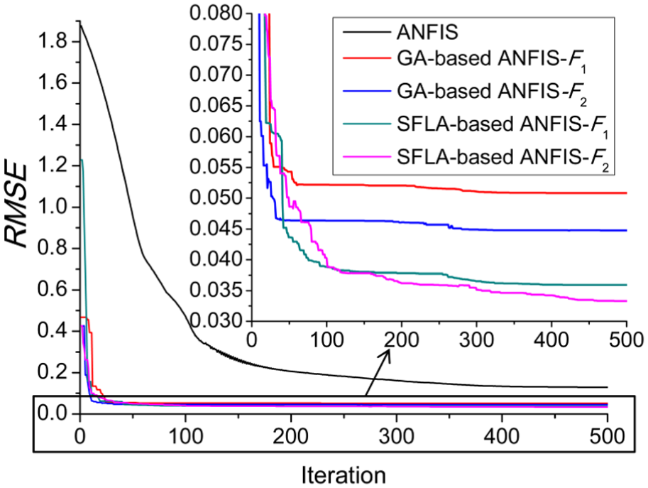
Convergence results of training errors achieved by different methods.

Figure 6.

Convergence results of checking errors achieved by different methods.

It is seen from Figures 5 and 6 that both of the SFLA-based ANFIS and GA-based ANFIS approaches perform significantly better than the ANFIS method in terms of convergence precision and convergence speed. Besides, compared with the GA-based ANFIS method, the SFLA-based ANFIS method achieves smaller training error and checking error no matter which fitness function is used. The reason why SFLA-based ANFIS is superior to GA-based ANFIS is probably that while GA falls into local extremes, SFLA still keeps searching till the best solution is obtained. Moreover, these two hybrid methods using the fitness function F₂ obtain smaller RMSE and RMSE_chk than those using the fitness function F₁.

It is shown from Figure 6 that the RMSE_chk in the ANFIS method initially decreases, seriously fluctuates, reaches a minimum, significantly increases and finally becomes almost steady. The phenomenon means that the system obtained with the ANFIS method learns noise during the training process which could affect the system generalization capability.³² Although the RMSE_chk slightly fluctuates in other methods in different extent, the overall tends are downward. In addition, it can be found from Figure 5 that in the beginning as the generation size increases, the RMSE in the hybrid methods with the fitness function F₂ does not decrease monotonically. This is not surprising, because the value of F₂ is affected not only by RMSE but also by RMSE_chk, although the effect brought by RMSE_chk is not much due to the large weighting coefficient w.

For more specific comparison, Table 5 shows the minimum and average errors given by different inverse modeling strategies. In the table, the numbers in the parentheses brackets are reduction ratios of the results of the hybrid methods versus the results of the ANFIS method. The numbers in the square brackets show reduction ratios of the results of SFLA-based ANFIS versus the results of GA-based ANFIS. As expected, among these methods, the SFLA-based ANFIS with the fitness value F₂ attains smallest minimum errors and average errors for both of training and checking data sets. There is high similarity between the comparison results of average errors and those of minimum errors, so here comparison results of the minimum errors are chosen to be discussed in detail. As for the training errors, the minimum RMSE obtained by SFLA-based ANFIS with F₁ (or F₂) is reduced by 29.36% (or 25.64%) compared with that obtained by GA-based ANFIS with F₁ (or F₂). Besides, the reduction ratio of minimum RMSE obtained by GA-based ANFIS with F₁ (or F₂) versus that obtained by ANFIS is 60.51% (or 65.21%). As for the checking errors, the minimum RMSE_chk given by SFLA-based ANFIS with F₁ (or F₂) achieves the reduction ratio of 28.25% (or 25.81%) versus that given by GA-based ANFIS with F₁ (or F₂) and reduction ratio of 96.59% (or 96.99%) versus that given by ANFIS. It can be deduced that such high reduction ratios for the RMSE_chk in the parentheses brackets in Table 5 are brought by the deterioration of the system generalization due to the ANFIS method.

Table 5.

Comparison of voltage errors obtained with different inverse modeling strategies.

Model output (voltage) comparison	Inverse modeling strategy
Model output (voltage) comparison	ANFIS	GA-based ANFIS with F₁	GA-based ANFIS with F₂	SFLA-based ANFIS with F₁	SFLA-based ANFIS with F₂
Minimum RMSE	0.12868	0.05082 (60.51%)	0.04477 (65.21%)	0.0359 (72.10%) [29.36%]	0.03329 (74.13%) [25.64%]
Average RMSE	0.12868	0.05378 (58.21%)	0.04859 (62.24%)	0.04008 (68.85%) [25.47%]	0.03459 (73.12%) [28.81%]
Minimum RMSE_chk	1.11463	0.05299 (95.25%)	0.04529 (95.94%)	0.03802 (96.59%) [28.25%]	0.03360 (96.99%) [25.81%]
Average RMSE_chk	1.11463	0.06838 (93.87%)	0.05031 (95.49%)	0.04215 (96.22%) [38.36%]	0.03515 (96.85%) [30.13%]

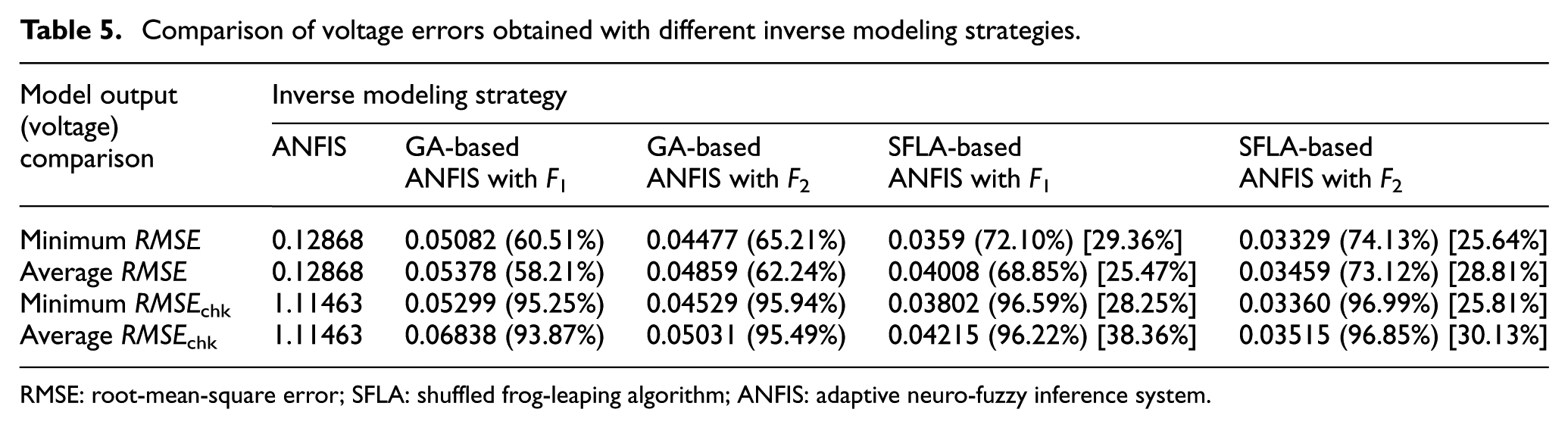
RMSE: root-mean-square error; SFLA: shuffled frog-leaping algorithm; ANFIS: adaptive neuro-fuzzy inference system.

To examine whether the performance of these hybrid inverse modeling methods is significantly different, four sets of statistical analyses are conducted with one-way ANOVA. In the first and second analyses, the factor (or source) is algorithm, that is, GA-based ANFIS and SFLA-based ANFIS strategies which adopt both fitness functions, and the responses are RMSE and RMSE_chk, respectively. In the third analysis, the factor is algorithm, that is, GA-based ANFIS and SFLA-based ANFIS, both of which use the fitness function F₁, and the response is F₁-related objective function Obj₁ which is equal to training error RMSE. In the fourth analysis, the factor is algorithm, that is, GA-based ANFIS and SFLA-based ANFIS, both of which use the fitness function F₂, and the response is F₂-related objective function Obj₂ which is defined as follows

Ob j_{2} = w \times RMSE + (1 - w) \times RMS E_{chk}

(23)

As mentioned above, w is equal to 0.8. According to equations (20) and (21), the smaller the Obj₁ and Obj₂ are, the larger the F₁ and F₂ are.

P values for these four sets of statistical analyses with one-way ANOVA are shown in Table 6. All p values are smaller than 0.05, which means that the performance of the compared algorithms is significantly different in terms of the corresponding response. Note that these small p values for the first and second analyses further manifest that different hybrid inverse modeling strategies with different fitness functions have notable effects on the values of RMSE and RMSE_chk.

Table 6.

P values for four sets of statistical analyses with one-way ANOVA.

Index	F statistic	p value
Obj ₁ versus algorithms with F₁	806.15	1.02638e−35
Obj ₂ versus algorithms with F₂	1082.52	3.25642e−39
RMSE versus algorithms with F₁ and F₂	728.53	4.64264e−75
RMSE _chk versus algorithms with F₁ and F₂	555.29	1.28928e−68

RMSE: root-mean-square error; ANOVA: analysis of variance.

For the third and fourth sets of statistical analyses, box plots in Figure 7(a) and (b), respectively, are utilized to visually determine the more effective algorithms. It is obvious that the median Obj₁ and Obj₂ of 30 runs obtained with SFLA-based ANFIS method are much smaller than those with GA-based ANFIS method. In order to compare these hybrid inverse modeling strategies in more detail, Table 7 shows the minimum error values (ME), average error values (AE), mean deviation (MD), and standard deviation (SD) for both of Obj₁ and Obj₂ given by GA-based ANFIS and SFLA-based ANFIS methods. MD and SD are defined as

MD = \frac{1}{N} \sum_{k = 1}^{N} | Obj (k) - \bar{Obj} (k) |

(24)

and

SD = \sqrt{\frac{1}{N} \sum_{k = 1}^{N} {(Obj (k) - \bar{Obj} (k))}^{2}}

(25)

respectively, where Obj (k) and $\bar{Obj} (k)$ denote the Obj₁ (Obj₂) of each run and the average Obj₁ (Obj₂), respectively. And N denotes the number of times each algorithm runs, N = 30.

Figure 7.

Box plots of different hybrid algorithms for two objective functions: (a) box plot of different algorithms for the objective function Obj₁ and (b) box plot of different algorithms for the objective function Obj₂.

Table 7.

Objective value comparison obtained with different hybrid inverse modeling strategies.

Objective value	Obj ₁(RMSE)		Obj ₂ (0.8RMSE + 0.2RMSE_chk)
Inverse modeling strategies	GA-based ANFIS-F₁	SFLA-based ANFIS-F₁	GA-based ANFIS-F₂	SFLA-based ANFIS-F₂
ME	0.05082	0.03590	0.04487	0.03335
AE	0.05378	0.04008	0.04894	0.03470
MD	0.00149	0.00144	0.00158	0.00092
SD	0.00176	0.00196	0.00210	0.00108

ME: minimum error; AE: average error; MD: mean deviation; SD: standard deviation; GA: genetic algorithm; RMSE: root-mean-square error; SFLA: shuffled frog-leaping algorithm; ANFIS: adaptive neuro-fuzzy inference system.

It is observed that all the values of ME, AE, MD, and SD achieved by SFLA-based ANFIS are smaller than those given by GA-based ANFIS, except the SD value in bold font in Obj₁ case. Therefore, in this study, SFLA-based ANFIS performs well in terms of robustness. It is noted that since both of the minimum and average objective values given by SFLA-based ANFIS strategy are smaller than GA-based ANFIS strategy, the former surpasses the latter in terms of convergence accuracy.

Moreover, the executive time for the traditional ANFIS, GA-based ANFIS, and SFLA-based ANFIS is compared. Searching the optimal solution of the ANFIS inverse model with EAs requires certain computational time. By MATLAB R2013b 64-bit by an Intel Core i7-4790 processor (3.6 GHz) with 16.0 GB RAM, under Windows 7, the average simulation time for 30 runs of GA-based ANFIS and SFLA-based ANFIS is approximately 30397.34 and 33106.43 s, respectively, while the optimization time is considerably reduced with traditional ANFIS (380.49 s). Although the runtime for SFLA-based ANFIS is about 1.09 and 87 times longer than that for GA-based ANFIS and traditional ANFIS, the accuracy of modeling and checking based on SFLA-based ANFIS has been improved in comparison with that based on the other two modeling strategies. On the other hand, since the inverse modeling of the MR damper is not a real-time problem, the simulation is performed based on off-line learning only. Therefore, the executive time is not a concern for the modeling problem. Compared with the executive time, how to improve the accuracy of the inverse model is the main concern.

Tables 8 and 9 list the optimal premise parameters and consequent parameters, respectively, optimized by the SFLA-based ANFIS method with fitness function F₂. The premise parameters are used to generate appropriate MFs as shown in Figure 8, while the consequent parameters are used to determine the fuzzy rules. Figure 9 compares the predicted voltage (output of the optimal inverse model) obtained with the SFLA-based ANFIS approach with F₂ and the target voltage for the checking data. The figure indicates that the predicted voltage and target voltage coincide very well, indicating that the optimized ANFIS has strong generalization capability.

Table 8.

Optimal premise parameters achieved by the SFLA-based ANFIS method with F₂.

Input variables	Optimal premise parameters
Input variables	a	b	c
Displacement	0.51060	10.00000	−3.50882
	2.67424	7.64321	0.07023
	0.86322	9.99986	3.88327
Velocity	32.99310	1.00000	−39.81852
	22.50889	10.00000	−15.00000
	41.60056	10.00000	45.00013
Damping force	222.67446	4.02014	−1933.57554
	1193.08930	2.94230	−647.77150
	951.18214	4.09714	1384.49300

SFLA: shuffled frog-leaping algorithm; ANFIS: adaptive neuro-fuzzy inference system.

Table 9.

Optimal consequent parameters achieved by the SFLA-based ANFIS method with F₂.

Rules	p	q	r	t
1	−3.63882 × 10⁻⁴	−2.46478 × 10⁻³	−7.27074 × 10⁻²	−3.19275 × 10⁻⁶
2	9.49135 × 10⁻³	8.53557 × 10⁻⁴	−2.85092 × 10⁻⁵	2.50814 × 10⁻²
3	−1.93889 × 10⁻¹	1.90260 × 10⁻²	−3.35751 × 10⁻³	−7.90073 × 10⁻²
4	−3.81986 × 10⁻⁴	−4.65675 × 10⁻³	−2.16362 × 10⁻¹	5.97392 × 10⁻⁵
5	9.13058 × 10⁻³	−4.34887 × 10⁻⁴	−1.67053 × 10⁻⁶	3.06672 × 10⁻²
6	−8.85544 × 10⁻²	1.89829 × 10⁻²	−4.74931 × 10⁻⁴	−2.29458 × 10⁻¹
7	−4.43421 × 10⁻⁵	−6.55707 × 10⁻⁶	−7.14354 × 10⁻³	9.79500 × 10⁻⁶
8	1.25075 × 10⁻²	3.93017 × 10⁻⁴	−3.76095 × 10⁻⁵	3.78481 × 10⁻²
9	3.98710 × 10⁻²	−4.80240 × 10⁻³	5.27297 × 10⁻⁴	1.33392 × 10⁻¹
10	6.86077 × 10⁻¹	−3.52901 × 10⁻⁴	1.29516 × 10⁻⁵	2.01299
11	6.79857 × 10⁻¹	1.82809 × 10⁻⁴	−6.22537 × 10⁻⁶	1.99440
12	6.74563 × 10⁻¹	−6.27395 × 10⁻⁴	1.27060 × 10⁻⁵	1.98852
13	6.79403 × 10⁻¹	1.58523 × 10⁻⁴	−5.95726 × 10⁻⁶	1.99393
14	6.82680 × 10⁻¹	−7.60003 × 10⁻⁵	2.71894 × 10⁻⁶	2.00244
15	6.83875 × 10⁻¹	1.84113 × 10⁻⁵	−4.65005 × 10⁻⁶	2.00404
16	−2.30392 × 10⁻¹	−1.60968 × 10⁻²	−2.02188 × 10⁻³	4.71708 × 10⁻¹
17	6.81284 × 10⁻¹	1.98324 × 10⁻⁵	−1.91646 × 10⁻⁶	1.99891
18	6.83385 × 10⁻¹	7.48963 × 10⁻⁵	−3.11758 × 10⁻⁶	2.00464
19	−7.88557 × 10⁻³	−1.47121 × 10⁻²	5.95555 × 10⁻⁵	1.58427
20	2.86562 × 10⁻²	−7.85867 × 10⁻⁴	−1.30738 × 10⁻⁶	3.85334
21	4.83874 × 10⁻²	7.82187 × 10⁻³	−4.87504 × 10⁻⁵	3.89862
22	3.83443 × 10⁻²	−3.49310 × 10⁻²	−5.41917 × 10⁻⁵	4.71129
23	1.24759 × 10⁻²	2.13095 × 10⁻⁴	6.40493 × 10⁻⁷	3.96482
24	8.63697 × 10⁻³	−7.17779 × 10⁻⁴	1.75127 × 10⁻⁵	3.93114
25	5.51356 × 10⁻¹	−1.20917 × 10⁻¹	−2.18341 × 10⁻³	1.91378 × 10⁻¹
26	2.25757 × 10⁻²	1.69815 × 10⁻³	1.45992 × 10⁻⁵	3.88167
27	1.36502 × 10⁻²	−9.68193 × 10⁻⁴	3.30876 × 10⁻⁶	3.92764

SFLA: shuffled frog-leaping algorithm; ANFIS: adaptive neuro-fuzzy inference system.

Figure 8.

Optimal membership functions obtained with the SFLA-based ANFIS method with F₂.

Figure 9.

Time histories of the predicted voltage given by the SFLA-based ANFIS inverse model and the target voltage for the checking data.

Finally, since the inverse models of the MR damper are developed to control the damping force, they are further validated with the RMSE values between the target damping force and predicted damping force calculated from the predicted voltage as shown in Table 10. RMSE and RMSE_chk in the table are the training and checking RMSE values for the damping force, respectively. As expected, the comparison results of the damping force among these modeling strategies have the similarity with those of the voltage in Table 7. It is clearly seen that the smallest minimum and average errors of damping force are achieved by the SFLA-based ANFIS method with fitness function F₂. The reduction ratios in the parentheses brackets clearly demonstrate that the hybrid strategies significantly outperform the ANFIS method in predicting the damping force. The reduction ratios in the square brackets show that the SFLA-based ANFIS method performs better than the GA-based ANFIS method no matter which fitness value is adopted.

Table 10.

Comparison of damping force errors obtained with different inverse modeling strategies.

Damping force comparison	Inverse modeling strategy
Damping force comparison	ANFIS	GA-based ANFIS with F₁	GA-based ANFIS with F₂	SFLA-based ANFIS with F₁	SFLA-based ANFIS with F₂
Minimum RMSE	34.73	12.08 (65.22%)	10.26 (70.46%)	7.88 (77.31%) [34.77%]	6.93 (80.05%) [32.46%]
Average RMSE	34.73	13.66 (60.67%)	11.4 (67.18%)	8.62 (75.18%) [36.90%]	8.34 (75.99%) [26.84%]
Minimum RMSE_chk	35.09	13.49 (61.56%)	10.42 (70.30%)	8.3 (76.35%) [38.47%]	7.03 (79.97%) [32.53%]
Average RMSE_chk	35.09	15.16 (56.80%)	11.74 (66.54%)	8.81 (74.89%) [41.89%]	8.43 (75.98%) [28.19%]

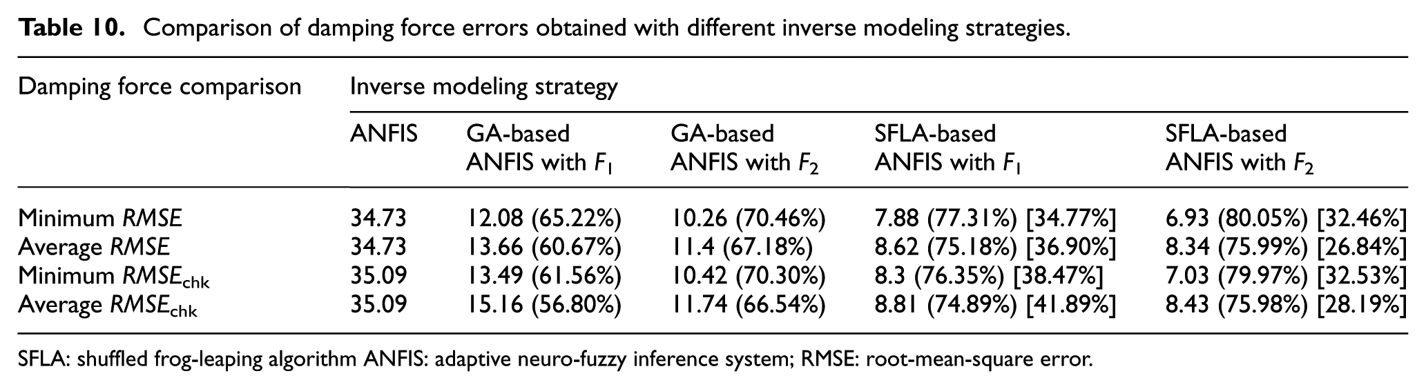
SFLA: shuffled frog-leaping algorithm ANFIS: adaptive neuro-fuzzy inference system; RMSE: root-mean-square error.

The comparison results of the minimum errors given by different strategies are shown as follows: GA-based ANFIS with F₁ (or F₂) outperforms ANFIS in terms of all RMSE values with reduction ratios of 65.22% (or 70.46%) for the minimum RMSE and 61.56% (or 70.30%) for the minimum RMSE_chk. As well, SFLA-based ANFIS using F₁ (or F₂) performs better than GA-based ANFIS using F₁ (or F₂) with reduction ratios of 34.77% (or 32.46%) for the minimum RMSE and 38.47% (or 32.53%) for the minimum RMSE_chk. Besides, it is interesting to find that the RMSE_chk of damping force given by the ANFIS method is not as large as expected. The reason is probably that the effect of deterioration of the system generalization on damping force is weakened during the nonlinear calculation of the damping force.

For a better visual comparison, Figure 10 illustrates the time histories of the predicted damping force obtained with the SFLA-based ANFIS method with F₂ and the target damping force for the checking data. It is clearly seen that there is almost no mismatch between them, indicating that the target damping force can be tracked very well by the predicted one.

Figure 10.

Time histories of the predicted damping force given by the SFLA-based ANFIS inverse model and the target damping force for the checking data.

Conclusion

Accurately controlling the MR damper has become an important issue in the field of the vibration control. To achieve this, it is necessary to model an accurate MR damper inverse model which can predict voltage input to the MR damper according to target damping force. In this article, a new hybrid strategy combining SFLA and ANFIS is proposed to achieve a more accurate MR damper inverse model. In the approach, SFLA is employed to determine the premise parameters of the ANFIS while whose consequent parameters are tuned by LSE. And the proposed SFLA-based ANFIS strategy is proposed to build the MR damper inverse model.

One contribution of this article is that SFLA is implemented for the first time for ANFIS model parameter determination. The second contribution is that EA (including SFLA and GA)-optimized ANFIS is first proposed to build the MR damper inverse model. The third contribution is using two-way ANOVA to study whether or not the parameters of SFLA, such as the number of the memeplexes m and population size N, have influences on the best solutions. And then the optimum combination of m and N is determined based on the statistical analysis. Furthermore, besides the fitness function F₁ related to the training RMSE value, for the sake of generalization capability of the ANFIS, another fitness function F₂ is proposed to slightly consider the checking accuracy on the basis of F₁. Finally, the statistical significance testing using one-way ANOVA is employed to prove the performances of the EA-based ANFIS strategies are significantly different. The simulation results are concluded as follows.

The comparison results of the voltage predicted by different MR damper inverse models show that the hybrid approaches including the SFLA-based ANFIS and GA-based ANFIS approaches are very promising, because they give advantages over the ANFIS method in terms of convergence accuracy and speed. Besides, the SFLA-based ANFIS method gives better results compared to the GA-based ANFIS method in terms of training accuracy and checking accuracy. In the hybrid strategies, two fitness functions are adopted and compared, and the results show that the hybrid strategies using the fitness function F₂ are superior to those using the fitness function F₁. Moreover, it is found that the ANFIS method not only gets stuck at local optima, but also learns noise during the system training phase, which is the reason why the system generalization deteriorates. However, the phenomenon of the generalization deterioration is avoided in the hybrid strategies.

Finally, further rigorous investigation is conducted to evaluate the performance of the inverse models on the prediction accuracy of the damping force. As expected, the SFLA-based ANFIS method performs best among these modeling strategies. It is interesting to find that the deterioration of the system generalization due to the ANFIS method affects the checking accuracy of the damping force not much, although it largely decreases the voltage checking accuracy.

Note that the SFLA-based ANFIS strategy can be extended to other application fields. Further study is to apply the proposed hybrid approach to vibration control strategy of a structural building with MR damper and show the improvement of controller performance. Moreover, future research work involves conducting an investigation of hybrid strategy combining improved SFLA or other advanced algorithms (or their variants) and ANFIS with higher accuracy for developing the MR damper inverse model.

Footnotes

Academic Editor: Amir Alavi

Declaration of conflicting interests

The author(s) declared no potential conflicts of interest with respect to the research, authorship, and/or publication of this article.

Funding

The author(s) disclosed receipt of the following financial support for the research, authorship, and/or publication of this article: This work was financially supported by Science and Technology Major Project of Fujian Province (2011HZ006-1), Special Funds for the University Development from Central Finance of China in 2012 and 2016, respectively, Construction of Scientific and Technological Innovation Platform of Fujian Province (2011H2008), and Science and Technology Project Founded by the Education Department of Fujian Province (JB13285).

References

Spencer

Jr Nagarajaiah

State of the art of structural control. J Struct Eng: ASCE 2003; 129: 845–856.

Ribakov

Agranovich

Using a limited set of MR dampers for improving structural seismic response. Struct Control Hlth 2015; 22: 615–630.

Atabak

Seiyed

Amir

AAK

. Neuro-fuzzy control strategy for an offshore steel jacket platform subjected to wave-induced forces using magnetorheological dampers. J Mech Sci Technol 2012; 26: 1179–1196.

Nugroho

. An adaptive neuro fuzzy hybrid control strategy for a semiactive suspension with magneto rheological damper. Adv Mech Eng 2014; 6: 487312-1–487312-11.

Arsava

Kim

Modeling of magnetorheological dampers under various impact loads. Shock Vib 2015; 2015: 905186-1–905186-20.

Shin

You

Hur

. Improvement of ride quality of railway vehicle by semiactive secondary suspension system on roller rig using magnetorheological damper. Adv Mech Eng 2014; 6: 298382-1–298382-10.

Salehi

Taghikhany

. Application of robust-optimum algorithms in semi-active control strategy for seismic protection of equipment. In: Proceedings of the 15th world conference on earthquake engineering, Lisbon, 24–28 September 2012, pp.24–28.

Wereley

Pang

Kamath

GM.

Idealized hysteresis modeling of electrorheological and magnetorheological dampers. J Intel Mat Syst Str 1998; 9: 642–649.

Spencer

Dyke

Sain

. Phenomenological model for magnetorheological dampers. J Eng Mech: ASCE 1997; 123: 230–238.

10.

Kwok

Nguyen

. A novel hysteretic model for magnetorheological fluid dampers and parameter identification using particle swarm optimization. Sensor Actuat A: Phys 2006; 132: 441–451.

11.

Choi

Lee

Park

YP.

A hysteresis model for the field-dependent damping force of a magnetorheological damper. J Sound Vib 2001; 245: 375–383.

12.

Tsang

RKL

Chandler

AM.

Simplified inverse dynamics models for MR fluid dampers. Eng Struct 2006; 28: 327–341.

13.

Salehi

Taghikhany

Fallah

AY.

Seismic protection of vulnerable equipment with semi-active control by employing robust and clipped-optimal algorithms. Int J Civ Eng 2014; 12: 413–428.

14.

Won

Sunwoo

Fuzzy modelling approach to magnetorheological dampers: forward and inverse model. Proc IMechE, Part I: J Systems and Control Engineering 2009; 223: 1055–1066.

15.

Wang

Liao

Modeling and control of magnetorheological fluid dampers using neural networks. Smart Mater Struct 2005; 14: 111–126.

16.

Bhowmik

Weber

Hogsberg

Experimental calibration of forward and inverse neural networks for rotary type magnetorheological damper. Struct Eng Mech 2013; 46: 673–693.

17.

Ekkachai

Tungpimolrut

Nilkhamhang

Force control of a magnetorheological damper using an elementary hysteresis model-based feedforward neural network. Smart Mater Struct 2013; 22: 115030-1–115030-9.

18.

Wang

. The neuro-fuzzy identification of MR damper. In: Proceedings of the 6th international conference on fuzzy systems and knowledge discovery, Tianjin, China, 14–16 August 2009, vol. 3, pp.464–468. New York: IEEE.

19.

Jang

JSR

. ANFIS: adaptive-network-based fuzzy inference system. IEEE T Syst Man Cyb 1993; 23: 665–684.

20.

Khalaj

MJ.

Application of ANFIS for modeling of layer thickness of chromium carbonitride coating. Neural Comput Appl 2014; 24: 685–694.

21.

Vella

WL.

Enhancing risk-adjusted performance of stock market intraday trading with neuro-fuzzy systems. Neurocomputing 2014; 141: 170–187.

22.

Eldessouki

Hassan

Adaptive neuro-fuzzy system for quantitative evaluation of woven fabrics’ pilling resistance. Expert Syst Appl 2015; 42: 2098–2113.

23.

Kharb

Shimi

Chatterji

. Modeling of solar PV module and maximum power point tracking using ANFIS. Renew Sust Energ Rev 2014; 33: 602–612.

24.

Mohanty

Parhi

DR.

Navigation of autonomous mobile robot using adaptive network based fuzzy inference system. J Mech Sci Technol 2014; 28: 2861–2868.

25.

Schurter

Roschke

. Fuzzy modeling of a magnetorheological damper using ANFIS. In: Proceedings of the 9th IEEE international conference on fuzzy systems, San Antonio, TX, 7–10 May 2000, vol. 1, pp.122–127. New York: IEEE.

26.

Zeinali

Mazlan

Abd Fatah

. A phenomenological dynamic model of a magnetorheological damper using a neuro-fuzzy system. Smart Mater Struct 2013; 22: 125013-1–125013-14.

27.

Haykin

Neural networks: a comprehensive foundation. 1st ed. Upper Saddle River, NJ: Prentice Hall, 1994.

28.

Holland

JH.

Adaption in natural and artificial systems. Cambridge, MA: MIT Press, 1976.

29.

Sarkheyli

Zain

Sharif

A multi-performance prediction model based on ANFIS and new modified-GA for machining processes. J Intell Manuf 2015; 26: 703–716.

30.

Djavareshkian

Esmaeili

Heuristic optimization of submerged hydrofoil using ANFIS–PSO. Ocean Eng 2014; 92: 55–63.

31.

Kumar

Mishra

MK.

Mitigation of voltage sags with phase jumps by UPQC with PSO-based ANFIS. IEEE T Power Deliver 2011; 26: 2761–2773.

32.

Oliveira

Schirru

Applying particle swarm optimization algorithm for tuning a neuro-fuzzy inference system for sensor monitoring. Prog Nucl Energ 2009; 51: 77–183.

33.

Jalali-Heravi

Asadollahi-Baboli

Quantitative structure-activity relationship study of serotonin (5-HT7) receptor inhibitors using modified ant colony algorithm and adaptive neuro-fuzzy interference system (ANFIS). Eur J Med Chem 2009; 44: 1463–1470.

34.

Eusuff

Lansey

KE.

Optimization of water distribution network design using the shuffled frog leaping algorithm. J Water Res Pl: ASCE 2003; 129: 210–225.

35.

Zhu

Zhang

WB.

An improved shuffled frog-leaping algorithm to optimize component pick-and-place sequencing optimization problem. Expert Syst Appl 2014; 41: 6818–6829.

36.

Gomez-Gonzalez

Jurado

Perez

Shuffled frog-leaping algorithm for parameter estimation of a double-cage asynchronous machine. IET Electr Power App 2012; 6: 484–490.

37.

Perez

Gomez-Gonzalez

Jurado

Estimation of induction motor parameters using shuffled frog-leaping algorithm. Electr Eng 2013; 95: 267–275.

38.

Naghizadeh

Vahidi

Hosseinian

SH.

Parameter identification of Jiles-Atherton model using SFLA. COMPEL 2012; 31: 1293–1309.

39.

Lin

Chen

SM.

A modified shuffled frog-leaping algorithm-based fuzzy controller for magnetorheological damper-building system. Int J Comput Appl T 2016; 53: 279–289.

40.

Pan

Xie

An effective shuffled frog-leaping algorithm for multi-objective flexible job shop scheduling problems. Appl Math Comput 2012; 218: 9353–9371.

41.

Cao

Zhao

. Swarm intelligence for atmospheric compensation in free space optical communication-modified shuffled frog leaping algorithm. Opt Laser Technol 2015; 66: 89–97.

42.

Arshi

Zolfaghari

Safaei

SM.

A multi-objective shuffled frog leaping algorithm for in-core fuel management optimization. Comput Phys Commun 2014; 185: 2622–2628.

43.

Hasanien

HM.

Shuffled frog leaping algorithm for photovoltaic model identification. IEEE T Sustain Energy 2015; 6: 509–515.

Optimal inverse magnetorheological damper modeling using shuffled frog-leaping algorithm–based adaptive neuro-fuzzy inference system approach