An algorithm to evaluate implementation cost for liveness-enforcing supervisors designed by deadlock prevention policy

Abstract

Deadlock prevention policy is widely used to design the liveness-enforcing supervisors because of its advantage that deadlocks are considered and solved in design and planning stages for flexible manufacturing systems modeled with Petri nets. However, how to evaluate the implementation cost of these liveness-enforcing supervisors is not done in the existing literature. This article proposes an algorithm to evaluate the implementation cost performance of different liveness-enforcing supervisors designed by deadlock prevention policy. By designing a multiple objective linear programming problem associated with two parameters (denoted as f₁ and f₂) to characterize the corresponding implementation costs for the added control places and the related input and out transitions and control arcs, the proposed algorithm first obtains the variable regions of f₁ and f₂ And then a satisfactory level coefficient (denoted as $\lambda$ ) concentrating on the optimal compromise solutions of f₁ and f₂ (denoted as f₁^* and f₂^*) is solved by a linear programming problem. As a result, the implementation cost performance of the corresponding liveness-enforcing supervisor can be indicated conveniently on the basis of the values of $\lambda$ , f₁^*, and f₂^*. The practical potential of the proposed algorithm is demonstrated via a theoretical analysis and several widely used examples from the existing literature.

Introduction

A flexible manufacturing system (FMS) is a computer-controlled configuration in which different operations are executed concurrently, and therefore, have to compete a limited number of shared resources such as robots, machines, storage devices, fixtures, conveyors, and so on.^1,2 Due to the competition of shared resources in a highly automated FMS, deadlocks that belong to highly undesirable phenomena occur frequently and then make the global or local FMS be blocked or crippled, leading to unnecessary economic cost or catastrophic results.^3–8 As a result, deadlock problems must be considered for designing an FMS. The deadlock control research has become the hot issues during the past two decades.^9–19

Petri nets have been widely used to model an FMS and to deal with deadlock problems because of their own features.^1,7 Three policies, called deadlock detection and recovery, deadlock avoidance, and deadlock prevention, respectively, are used to deal with deadlock problems in FMSs. Among them, deadlock prevention policy (DPP) is widely used to design the liveness-enforcing supervisors to cope with deadlocks in FMSs due to major advantages that its execution requires no run-time cost and is carried out off-line, implying that deadlocks are considered and solved in design and planning stages for FMSs. Two methods belonged to DPP, siphon-based method (SBM) and reachability graph-based method (RGBM), are currently used to design the liveness-enforcing supervisors in deadlock control research in terms of behavioral permissiveness (BP), structural complexity (SC), and computational complexity (CC). As a structural object of a Petri net, siphon is closely related to deadlocks in Petri net models. Many scholars focus on solving and controlling the siphons and have developed a large number of deadlock control policies (DCPs) using SBM.^1,20 Ezpeleta and colleagues,^4,10 Li and colleagues,^{1,2,7,14,15,21–26} Huang et al.,^5,11 Chao,^3,9 Piroddi et al., ¹⁸ and Park and Reveliotis, ¹⁷ and so on are the leading figures in this research field due to their significant contributions. Among these representative DCPs, E-policy^4,10 and LZ-policy^21–24,26 adopt the complete siphon enumeration method (CSEM) to solve all siphons causing deadlocks. E-policy adds a control place (CP) to each emptied siphon to prevent itself from being emptied and then obtains a much more structurally complex liveness-enforcing supervisor than the plant net model, leading to the fact that the performance of the corresponding liveness-enforcing supervisor is not ideal in terms of BP, SC, and CC. By the concept of elementary siphons, LZ-policy only adds the CPs to the solved elementary siphons and their dependent siphons that cannot meet the controllability and then achieves a liveness-enforcing supervisor with a relative simple structure, which reduces SC of the corresponding liveness-enforcing supervisor to some degree than E-policy, but BP and CC of the corresponding liveness-enforcing supervisor are not improved any more. Using mixed integer programming (MIP) and the partial siphon enumeration method (PSEM), C-policy,^3,9 H-policy,^5,11 PR-policy, ¹⁷ P-policy, ¹⁸ LL-policy,^6,13,27–30 and L-policy ¹⁶ focus on solving these siphons that definitely cause deadlocks and then make them max-controlled or max′-controlled by adding CPs, resulting in the fact that the corresponding liveness-enforcing supervisors with a simpler structure and more permissive behavior can be yielded usually and the computational efficiency of these DCPs are more efficient in comparison to E-policy and LZ-policy. In general, CC and SC of liveness-enforcing supervisors constructed by SBM are relatively ideal but BP is not optimal (maximally permissive).

On the other hand, RGBM are used to deal with deadlocks in Petri net models as well. It is known that a reachability graph (RG) consists of deadlock zone (DZ) including deadlocks and critical bad states that inevitably lead to deadlocks, and a deadlock-free-zone (DFZ) representing the good states of an RG. The early representative scholars, Uzam and colleagues,^19,31 design the DCPs to ensure the corresponding liveness in terms of RG of the Petri net. That is to say, their DCPs can prevent the system from entering DZ, while making sure that every state within DFZ can still be reached. So UZ-policy ¹⁹ is previously considered to be optimal in terms of their BP, that is, maximally permissive behavior. However, its computational load is too heavy and SC of the corresponding liveness-enforcing supervisors is not reduced any more. By the identifying method in Li and Li, ²⁷ a few reductant CPs can be found in the live-controlled Petri net systems obtained by UZ-policy. Accordingly, using minimal covering set ${\mathcal{M}}_L^{*}$ of legal markings, minimal covered set ${\mathcal{M}}_F^{*}$ of first-met bad markings (FBMs) with RGBM, and the idea of structural minimality of optimal supervisors, Chen and colleagues^32–36 also obtain the liveness-enforcing Petri net supervisors with maximally permissive behavior, but CC and SC of the corresponding liveness-enforcing supervisors constructed by CL-policy^32–35 are observably improved than those constructed by UZ-policy. Especially, Chen et al. ³⁶ propose the concept of interval inhibitor arcs and its application to the optimal supervisory control of Petri nets. Both maximally permissive behavior and simpler structure for the Petri net supervisors are achieved than some net models that cannot be optimally controlled by pure net supervisor. Lately, by the methods of multiobjective integer programming and eliminating redundant constraint, Huang et al.^12,37,38 achieve the optimal and structurally minimal Petri net supervisors and the computational load of HZ-policy ³⁸ is relatively low. The academic results from both these scholars and other unmentioned researchers enrich DCPs and the relevant deadlock control theories derived from a Petri net formalism. A common point of the above DCPs is that BP, SC, and CC of the liveness-enforcing supervisors are sufficiently considered during the corresponding design stage. However, how to further evaluate the implementation cost performance (ICP) of these liveness-enforcing supervisors constructed by the above DCPs is not taken into account in the existing literature.

Considering the shortcoming mentioned in the above DCPs, this article proposes a novel algorithm to evaluate the ICP of different kinds of liveness-enforcing supervisors designed by the existing DCPs in the literature. As for a liveness-enforcing supervisor in the live-controlled Petri net system, its evolving behavior characterization can be described by the theories in Li and Zhou^1,2 and Qin et al. ³⁹ and analyzed by INA ⁴⁰ practically. So it can be inferred that its ICP mainly involves several factors associated with the added CPs, the related input and out transitions, and input and output control arcs linking CPs with input and out transitions, including their number and their initial markings for CPs, firing times (occurrences) for input and output transitions, and the number and weight values for input and output control arcs. It is known that the added CPs represent programmable logic controllers (PLCs) that can analyze and judge the information from sensors and then issue the proper instructions to actuators, similar to the brain of a person. Their number and initial markings of CPs describe the number and processing capacity of the PLCs. The related input and out transitions and input and output control arcs denote sensors, actuators, input and output signal circuits, respectively. The firing times for input and output transitions indicate that sensors and actuators are in active states, respectively. Meanwhile, the number and weight values for input and output control arcs represent the number and the capacity of sending and receiving signals for the corresponding input and output signal circuits. Hence, an evaluation problem of the ICP of a liveness-enforcing supervisor is associated with a number of factors above. In this article, first, we introduce the first parameter $f_1$ concerning with the number and initial markings of the added CPs to characterize implementation cost for CPs. Accordingly, the second parameter $f_2$ associated with firing times (occurrences) of input and output transitions and the number and weight values of input and output control arcs is introduced to describe synthetical implementation cost for sensors, actuators, and the corresponding input and output signal circuits. As a result, an ICP evaluation problem relies on solving $f_1$ and $f_2$ for a liveness-enforcing supervisor, and the solutions of $f_1$ and $f_2$ are attributed to a multiple objective linear programming problem (MOLPP) that is depicted in section “Optimal compromise solutions for the ICP of a liveness-enforcing supervisor.”

Partially enlightened by the methods in Li and Zhou, ²² Huang et al., ³⁷ Baky, ⁴¹ and Pourkarimi et al., ⁴² the proposed algorithm including an MOLPP is designed and then executed in two stages. At the first stage, solving an MOLPP with $f_1$ and $f_2$ twice via equations (1)–(4) in section “An MOLPP associated with f₁ and f₂,” two solutions of $f_1$ (denoted as $f_1^{*}{,}_1$ and $f_1^{*}{,}_2$ ) and $f_2$ (denoted as $f_2^{*}{,}_1$ and $f_2^{*}{,}_2$ ) are separately yielded, and then the variable regions of $f_1$ and $f_2$ and the membership functions of $f_1$ and $f_2$ can be determined, respectively. According to the theories in Baky, ⁴¹ Pourkarimi et al., ⁴² and Leung, ⁴³ the optimal solution for an objective function may not be an optimal solution for the other objective functions, for example, the optimal solution of $f_1$ may not be an optimal solution for $f_2$ , and vice versa. So a satisfactory level coefficient (denoted as $\lambda$ ) that can characterize the optimal compromise solutions for $f_1$ and $f_2$ (denoted $f_1^{*}$ and $f_2^{*}$ ) is introduced and a linear programming problem (LPP) with $\lambda$ is designed at the second stage. Based on the results obtained from the first stage and adding some new constraints, an LPP with $\lambda$ is solved through equations (5)–(9) in section “A LPP associated with an ICP evaluation,” and the corresponding optimal compromise solutions of $f_1^{*}$ and $f_2^{*}$ are yielded as well. As a result, the ICP evaluation of a liveness-enforcing supervisor is shown in terms of the values of $\lambda$ , $f_1^{*}$ , and $f_2^{*}$ .

The remainder of this work is organized as follows. Section “Some relevant basic concepts of Petri nets” reviews preliminaries of Petri nets that are used throughout this work. Definitions of three weight coefficients (denoted as ${\alpha }_{V_k}$ , ${\beta }_{V_k}$ , and ${\gamma }_{V_k}$ ) associated with $f_1$ and $f_2$ is given in section “Three weight coefficients ${\alpha }_{V_k}$ , ${\beta }_{V_k}$ , and ${\gamma }_{V_k}$ .” By means of analysis of the evolving behavior characterization of a liveness-enforcing supervisor^1,2,39 and the theories in Baky, ⁴¹ Pourkarimi et al., ⁴² and Leung ⁴³ an MOLPP considering $f_1$ and $f_2$ as the objective functions is first designed in section “An MOLPP associated with f₁ and f₂.” By adding some new constraints, section “A LPP associated with an ICP evaluation” presents a LPP with $\lambda$ accordingly. A novel algorithm to evaluate the ICP of the liveness-enforcing supervisors constructed by SBM or RGBM is developed in section “An iterative ICP evaluating algorithm,” which indicates how about the ICP of a liveness-enforcing supervisor is in terms of the values of $\lambda$ , $f_1^{*}$ , and $f_2^{*}$ . In section “Case study,” several widely used examples from the aboveliterature^{2,4,11–13,17,19,21,22,30,32,33} are demonstrated the applications of the proposed algorithm, and a qualitative evaluation for the ICP comparison of a liveness-enforcing supervisor with the other ones is offered via this case study. Finally, Section “Conclusion” concludes this article.

Preliminaries

Some relevant basic concepts of Petri nets

A Petri net is a four-tuple $N=(P,T,F,W)$ , where P and T are finite and non-empty sets. P is a set of places and T is a set of transitions with $P\cup T\ne Ø$ and $P\cap T=Ø$ . $F\subseteq (P\times T)\cup (T\times P)$ is called the flow relation or the set of directed arcs. $W:(P\times T)\cup (T\times P)\to \mathbb{N}$ is a mapping that assigns a weight to an arc: $W(x,y)>0$ if $(x,y)\in F$ , and $W(x,y)=0$ otherwise, where $x,y\in P\cup T$ and ℕ denotes the set of non-negative integers. $N=(P,T,F,W)$ is called an ordinary net, denoted as $N=(P,T,F)$ , if $\forall f\in F,W(f)=1$ . $N=(P,T,F,W)$ is called a generalized net, if $\exists f\in F,W(f)>1$ . Given a node $x\in P\cup T$ , ${}^{•}x=\{y\in P\cup T|(y,x)\in F\}$ is called the preset of x, while $x^{•}=\{y\in P\cup T|(x,y)\in F\}$ is called the post-set of x. A marking is a mapping $M:P\to \mathbb{N}$ . $(N,M_0)$ is called a marked Petri net or a net system. The set of markings reachable from M in N is denoted as $R(N,M)$ . Incidence matrix $[N]$ of net N is a $|P|\times |T|$ integer matrix with $[N](p,t)=W(t,p)-W(p,t)$ , where $|P|$ and $|T|$ denote the number of places and transitions in N, respectively. Given a Petri net $(N,M_0)$ , $t\in T$ is live under $M_0$ if $\forall M\in R(N,M_0),\exists M\prime \in (N,M),M\prime [t〉.$ $(N,M_0)$ is live if $\forall t\in T,t$ is live under $M_0$ . $(N,M_0)$ is dead under $M_0$ if $/\exists t\in T,M_0[t〉$ . $(N,M_0)$ is deadlock-free (weakly live) if $\forall M\in R(N,M_0),\exists t\in T,M[t〉$ . ¹

A liveness-enforcing supervisor is denoted by $(N\prime ,M{\prime }_0)$ , where $N\prime =(V,T_{\mathrm{input}}\cup T_{\mathrm{output}},F\prime ,W\prime )$ , $V=\{V_1,V_2,\dots ,V_k\}$ is the set of the added CPs, $T_{\mathrm{input}}\cup T_{\mathrm{output}}\subset T$ is the set of input and output transitions of the added CPs, $F\prime$ is the set of input and out control arcs that are used to link the added CPs to $T_{\mathrm{input}}$ ( ${}^{•}V$ ) and $T_{\mathrm{output}}$ ( $V^{•}$ ) in the liveness-enforcing supervisor $(N\prime ,M{\prime }_0)$ , $W\prime$ denotes the set of weight values of input and out control arcs in the liveness-enforcing supervisor $(N\prime ,M{\prime }_0)$ , and $k\in {\mathbb{N}}^{+}=\{1,2,\dots \}$ . Then, the live-controlled Petri net system is denoted as $(N^{*},M_0^{*})$ with $N^{*}=(P^{*},T,F^{*},W^{*})$ , where $P^{*}=P\cup V,F^{*}=F\cup F\prime$ , and $W^{*}=W\cup W\prime$ . Incidence matrix $[N^{*}]$ of the live-controlled net $N^{*}$ is a $|P^{*}|\times |T|$ integer matrix with $[N^{*}](p,t)=W^{*}(t,p)-W^{*}(p,t)$ , where $|P^{*}|$ and $|T|$ denote the total number of places and transitions in $N^{*}$ , respectively, $\forall p\in P^{*}$ .

Definition 1

Let $N=(P,T,F,W)$ be a net and $\sigma$ be a finite sequence of transitions. ¹ The Parikh vector of $\sigma$ is $\overrightarrow{\sigma }$ : $T\to \mathbb{N}$ which maps t in T to the number of occurrences of t in $\sigma$ .

Three weight coefficients ${\alpha }_{V_k},{\beta }_{V_k},$ and ${\gamma }_{V_k}$

From Li and Zhou,^1,2 and Ezpeleta and Recalde ¹⁰ , the interrelation between markings and numbers of transition occurrences in a transition sequence can be expressed by the state equation of an original Petri net $(N,M)$ : $M(p)=M_0(p)+[N]\overrightarrow{\sigma },\forall p\in P$ . Clearly, as for a live-controlled Petri net system $(N^{*},M_0^{*})$ , we have $M^{*}(p)={M^{*}}_0(p)+[N^{*}]\overrightarrow{{\sigma }^{*}},\forall p\in P^{*}$ , called the state equation of $(N^{*},M_0^{*})$ , which can express the interrelation between markings and numbers of transition occurrences in ${\sigma }^{*}$ in $N^{*}$ . In this article, for all input and output transitions of each $V_k$ , we use $|t_{\mathrm{input}},V_k|$ and $|t_{\mathrm{output}},V_k|$ to denote the total number of input and output transition occurrences in ${\sigma }^{*}$ for each $V_k$ in $N^{*}$ , respectively. That is to say, $|t_{\mathrm{input}},V_k|$ ( $|t_{\mathrm{output}},V_k|$ ) denotes the firing times of input (out) transitions linking with each $V_k$ in $N^{*}$ . Clearly, the solutions of $|t_{\mathrm{input}},V_k|$ and $|t_{\mathrm{output}},V_k|$ can be obtained from ${\sigma }^{*}$ by solving $M^{*}(p)={M^{*}}_0(p)+[N^{*}]\overleftarrow{{\sigma }^{*}}$ .

As stated previously, on the basis of analyzing the evolving behavior characterization of a liveness-enforcing supervisor,^1,2,39 its ICP involves several factors associated with the added CPs and the related input and output transitions, including their number and their initial markings for CPs, firing times (occurrences) for input and output transitions ( $|t_{\mathrm{input}},V_k|$ and $|t_{\mathrm{output}},V_k|$ ), and the number and weight values for input and output control arcs. Since $|t_{\mathrm{input}},V_k|$ and $|t_{\mathrm{output}},V_k|$ can be found from ${\sigma }^{*}$ by solving $M^{*}(p)={M^{*}}_0(p)+[N^{*}]\overrightarrow{{\sigma }^{*}}$ , we propose three weight coefficients ${\alpha }_{V_k},{\beta }_{V_k},\mathrm{and}{\gamma }_{V_k}$ concerning the above factors except firing times for input and output transitions, which are defined as below, respectively.

Definition 2

$(N\prime ,M{\prime }_0)$ is the corresponding liveness-enforcing supervisor in a live-controlled net $(N^{*},M_0^{*})$ and $V=\{V_1,V_2,\dots ,V_k\}$ is the set of the added CPs in $(N\prime ,M{\prime }_0)$ . Let ${\alpha }_{V_k}$ be a weight coefficient with respect to the marking of each $V_k$ , where ${\alpha }_{V_k}=(M_0(V_k))/(\sum _{k=1}^{|V|}{M}_0(V_k))$ , $|V|$ denotes the total number of the added CPs, $k,|V|\in {\mathbb{N}}^{+}=\{1,2,\dots \}$ .

Definition 3

For $V=\{V_1,V_2,\dots ,V_k\}$ in $(N\prime ,M{\prime }_0)$ , $T_{\mathrm{input}}={}^{•}V={{}^{•}V}_1\cup {{}^{•}V}_2\cup \dots \cup {{}^{•}V}_k$ is the set of input transitions of the added CPs in $(N\prime ,M{\prime }_0)$ . Let ${\beta }_{V_k}$ be a weight coefficient with respect to implementation cost of input control arcs of each $V_k$ , where ${\beta }_{V_k}=\frac{\sum _{t_{\mathrm{input}}\in {{}^{•}V}_k}W(t_{\mathrm{input}},V_k)}{\sum _{k=1}^{|V|}(\sum _{t_{\mathrm{input}}\in {{}^{•}V}_k}W(t_{\mathrm{input}},V_k))},\forall t_{\mathrm{input}}\in {{}^{•}V}_k,\forall {{}^{•}V}_k\in T_{\mathrm{input}}$

Definition 4

For $V=\{V_1,V_2,\dots ,V_k\}$ in $(N\prime ,M{\prime }_0)$ , $T_{\mathrm{output}}=V^{•}=V_1^{•}\cup V_2^{•}\cup \cdots \cup V_k^{•}$ is the set of output transitions of the added CPs in $(N\prime ,M{\prime }_0)$ . Let ${\gamma }_{V_k}$ be a weight coefficient with respect to implementation cost of output control arcs of each $V_k$ , where ${\gamma }_{V_k}=\frac{\sum _{t_{\mathrm{output}}\in {V_k}^{•}}W(t_{\mathrm{output}},V_k)}{\sum _{k=1}^{|V|}(\sum _{t_{\mathrm{output}}\in {V_k}^{•}}W(t_{\mathrm{output}},V_k))},\forall t_{\mathrm{output}}\in {V_k}^{•},\forall {V_k}^{•}\in T_{\mathrm{output}}$

The physical meanings of ${\alpha }_{V_k},{\beta }_{V_k},\mathrm{and}{\gamma }_{V_k}$ can be explained intuitively as follows. From Li and Zhou, ¹ Huang, ¹² and Liu and Barkaoui, ²⁰ the important core part of an FMS is a highly automatic control system (ACS) with a number of PLCs, sensors, actuators, and the related circuits of sending and receiving signals, and so on. Obviously, each PLC, sensor, actuator as well as circuit of sending and receiving signals plays a different role in an ACS. The value of ${\alpha }_{V_k}$ for a PLC describes how about its processing capacity and influence are among a set of PLCs in an ACS. In addition, for a PLC ( $V_k$ ), there are more than one circuit of sending signals from more than one sensor to it in general. ${\beta }_{V_k}$ presents how about the influence of all signal input circuits from sensors to a $V_k$ among a set of the signal input circuits of all PLCs (V) in an ACS. Similarly, there are more than one circuit of receiving signals from more than one actuator to a PLC. ${\gamma }_{V_k}$ represents how about the corresponding influence of all signal output circuits from actuators to a $V_k$ among a set of the signal output circuits of all PLCs (V) in an ACS. In short, the higher values of ${\alpha }_{V_k},{\beta }_{V_k},\mathrm{and}{\gamma }_{V_k}$ mean the stronger effects of a PLC ( $V_k$ ) and its signal input and out circuits linking with the corresponding sensors and actuators to an ACS in an FMS.

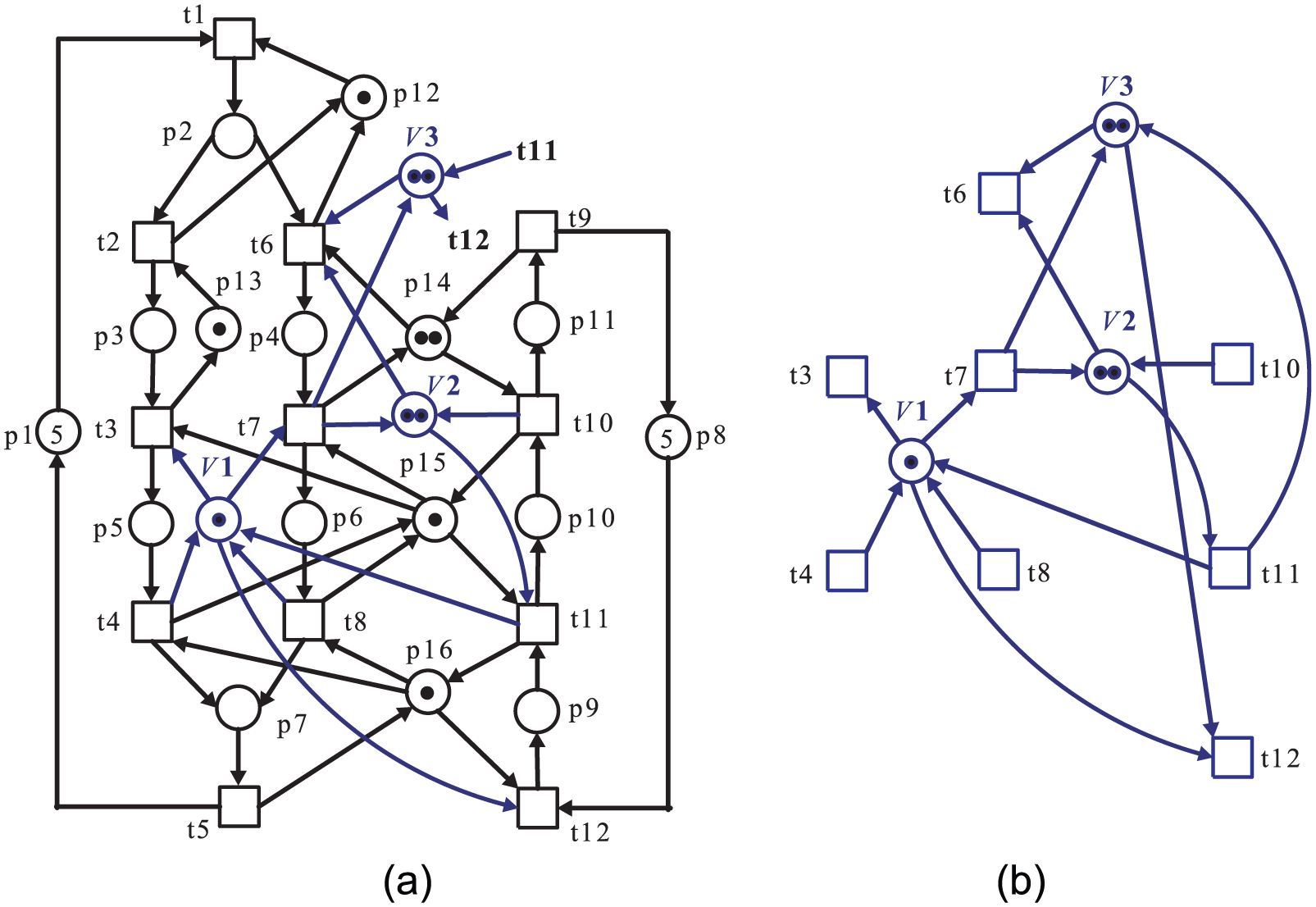
For example, Figure 1(a) and (b) ²⁹ shows the live-controlled S³PR system and the corresponding liveness-enforcing supervisor, respectively, where $P=\{p_1,p_2,\dots ,p_{16}\}$ , $T=\{t_1,t_2,\dots ,t_{12}\}$ , and $V=\{V_1,V_2,V_3\}$ .

Figure 1.

(a) A live-controlled S³PR system $(N^{*},M_0^{*})$ and (b) the corresponding liveness-enforcing supervisor $(N\prime ,M{\prime }_0)$ .

From the above description in section “Some relevant basic concepts of Petri nets,” we have $T_{\mathrm{input}}={}^{•}V{=}^{•}{V}_1{\cup }^{•}{V}_2{\cup }^{•}{V}_3=\{t_4,t_7,t_8,t_{10},t_{11}\}$ , $T_{\mathrm{output}}=V^{•}={V_1}^{•}\cup {V_2}^{•}\cup {V_3}^{•}=\{t_3,t_6,t_7,t_{11},t_{12}\}$ . From Definition 2–4, for $V_1$ , $V_2$ , and $V_3$ , ${\alpha }_{V_1}=(1/5)=0.2$ , ${\alpha }_{V_2}={\alpha }_{V_3}=(2/5)=0.4$ , ${\beta }_{V_1}=(3/7)=0.43$ , ${\beta }_{V_2}={\beta }_{V_3}=(2/7)=0.285$ , ${\gamma }_{V_1}=(3/7)=0.43$ , and ${\gamma }_{V_2}={\gamma }_{V_3}=(2/7)=0.285$ can be obtained, respectively. Moreover, for $V_1$ , $|t_{\mathrm{input}},V_1|$ and $|t_{\mathrm{output}},V_1|$ denote the total number of occurrences for $\{t_4,t_8,t_{11}\}$ and $\{t_3,t_7,t_{12}\}$ in ${\sigma }^{*}$ , respectively. Similarly, for $V_2$ ( $V_3$ ), $|t_{\mathrm{input}},V_2|$ and $|t_{\mathrm{output}},V_2|$ ( $|t_{\mathrm{input}},V_3|$ and $|t_{\mathrm{output}},V_3|$ ) denote the total number of occurrences for $\{t_7,t_{10}\}$ and $\{t_6,t_{11}\}$ ( $\{t_7,t_{11}\}$ and $\{t_6,t_{12}\}$ ) in ${\sigma }^{*}$ in $N^{*}$ , respectively. By programming the interrelation between markings and numbers of transition occurrences of $M^{*}(p)={M^{*}}_0(p)+[N^{*}]\overrightarrow{{\sigma }^{*}}$ of a live-controlled S³PR system depicted in Figure 1(a) with LinGo, ⁴⁴ the values of $|t_{\mathrm{input}},V_1|$ , $|t_{\mathrm{output}},V_1|$ , $|t_{\mathrm{input}},V_2|$ , $|t_{\mathrm{output}},V_2|$ , $|t_{\mathrm{input}},V_3|$ , and $|t_{\mathrm{output}},V_3|$ can be obtained from $\overrightarrow{{\sigma }^{*}}$ , respectively, that is, 0, 1, 1, 3, 1, and 3.

Optimal compromise solutions for the ICP of a liveness-enforcing supervisor

An MOLPP associated with f₁ and f₂

As stated above, in this study, we introduce the first parameter $f_1$ concerning with the number of the added CPs labeled different markings to characterize the synthetical implementation cost for all CPs. So an objective function $min{f}_1=\sum _{k=1}^{|V|}{\alpha }_{V_k}{M}^{*}(V_k)$ is first designed and subject to $M^{*}(p)={M^{*}}_0(p)+[N^{*}]\overrightarrow{{\sigma }^{*}}$ , where minimizing $f_1$ means the more economic implementation cost for the all added CPs. That is to say, $f_1$ describes the synthetical implementation cost for all CPs with different processing capacities when the corresponding liveness-enforcing supervisor acts to eliminate deadlocks. The lower the value of $f_1$ , the more economic the synthetical implementation cost for all CPs is. Accordingly, the second parameter $f_2$ associated with firing times (occurrences) of input and output transitions and the number and weight values of input and output control arcs is also introduced to describe the synthetical implementation cost for sensors, actuators, and the corresponding input and output signal circuits. Another objective function: $min{f}_2=\sum _{k=1}^{|V|}({\beta }_{V_k}|t_{\mathrm{input}},V_k|+{\gamma }_{V_k}|t_{\mathrm{output}},V_k|)$ is constructed and subject to the same constraints as well, where minimizing $f_2$ means that the related sensors, actuators, and the corresponding input and output signal circuits are in active states with lower or more economic implementation cost in an ACS. In other words, $f_2$ characterizes the synthetical implementation cost for the related sensors, actuators, and the corresponding input and output signal circuits when the corresponding liveness-enforcing supervisor acts to eliminate deadlocks. Similarly, the lower the value of $f_2$ , the more economic or the lower the synthetical implementation cost for all sensors, actuators, and the corresponding input and output signal circuits is.

Therefore, by means of the ideas in Baky, ⁴¹ Pourkarimi et al., ⁴² and Leung ⁴³ $f_1$ and $f_2$ are considered as the objective functions of the key MOLPP, which is described as follows

$$\min f_1={\displaystyle \sum _{k=1}^{\left|V\right|}}{\alpha }_{V_k}{M}^{*}(V_k)$$

(1)

$$\min f_2={\displaystyle \sum _{k=1}^{\left|V\right|}}({\beta }_{V_k}|t_{input}\mathrm{,}{V}_k|+{\gamma }_{V_k}|t_{output}\mathrm{,}{V}_k|)$$

(2)

s. t.

$$M^{*}(p)=M_0^{*}(p)+[N^{*}]\overrightarrow{{\sigma }^{*}}$$

(3)

$$M^{*}(p)\ge 0,\forall p\in P^{*}\mathrm{,}\forall V_k\in V\mathrm{,}\overrightarrow{{\sigma }^{*}}\ge 0$$

(4)

It is seen that the proposed ICP problem decides the economic or low cost for the actual operation of a liveness-enforcing supervisor. So we minimize two objective functions $f_1$ and $f_2$ that are subject to the given set of constraints from the state equation of a live-controlled Petri net system $(N^{*},M_0^{*})$ and others. ¹ In order to solve the optimal solutions of $f_1$ and $f_2$ , it needs to execute the above MOLPP in two steps. At the first step, for objective $f_1$ , solving equation (1) under the constraint conditions equations (3) and (4), we have the optimal solution of $f_1$ (denoted as $f_1^{*}{,}_1$ ) with the corresponding optimal solutions of $M^{*}(V_k){,}_1$ , $|t_{\mathrm{input}},V_k{|}^{*}{,}_1$ , and $|t_{\mathrm{output}},V_k{|}^{*}{,}_1$ . Then, the corresponding optimal solution of $f_2$ (denoted as ${f_2}^{*}{,}_1$ ) can be obtained by substituting the values of $|t_{\mathrm{input}},V_k{|}^{*}{,}_1$ and $|t_{\mathrm{output}},V_k{|}^{*}{,}_1$ into equation (2). At the second step, similarly, for objective $f_2$ , solving equation (2) under the same constraint conditions, the optimal solution of $f_2$ (denoted as $f_2^{*}{,}_2$ ) with the corresponding optimal solutions of $M^{*}(V_k){,}_2$ , $|t_{\mathrm{input}},V_k{|}^{*}{,}_2$ , and $|t_{\mathrm{output}},V_k{|}^{*}{,}_2$ can be obtained. Accordingly, we have the corresponding optimal solution of $f_1$ (denoted as $f_1^{*}{,}_2$ ) by substituting the values of $M^{*}(V_k){,}_2$ into equation (1).

Analyzing the values of ${f_1}^{*}{,}_1,{f_1}^{*}{,}_2$ , ${f_2}^{*}{,}_1$ , and ${f_2}^{*}{,}_2$ , we can determine the variable regions of $f_1$ and $f_2$ , respectively, that is, $f_1\in [{f_1}^L,{f_1}^H]$ and $f_2\in [{f_2}^L,{f_2}^H]$ , where ${f_1}^L=min\{{f_1}^{*}{,}_1,{f_1}^{*}{,}_2\}$ , ${f_1}^H=max\{{f_1}^{*}{,}_1,{f_1}^{*}{,}_2\}$ , ${f_2}^L=min\{{f_2}^{*}{,}_1,{f_2}^{*}{,}_2\}$ , and ${f_2}^H=max\{f_2^{*}{,}_1,f_2^{*}{,}_2\}$ . Moreover, $d_1$ and $d_2$ , called the extension indexes of $f_1$ and $f_2$ , can be determined, respectively, where $d_1=f_1^H-f_1^L$ and $d_2=f_2^H-f_2^L$ . Meanwhile, the membership functions of $f_1$ and $f_2$ , denoted as $G_1(M)$ and $G_2(t)$ , are further derived, respectively, where $G_1(M)=[f_1^H-f_1]/d_1,f_1^H-d_1\le f_1\le f_1^H$ , $G_2(t)=[f_2^H-f_2]/d_2,f_2^H-d_2\le f_2\le f_2^H$ . The variations of $G_1(M)$ with $f_1$ and $G_2(t)$ with $f_2$ are depicted in Figure 2(a) and (b), respectively.

Figure 2.

(a) Variation of $G_1(M)$ with $f_1$ and (b) variation of $G_2(t)$ with $f_2$ .

An LPP associated with an ICP evaluation

From the results in section “An MOLPP associated with f₁ and f₂,” the variable regions of $f_1$ and $f_2$ are obtained. Since the optimal solution for $f_1$ may not be an optimal solution for $f_2$ , and vice versa, it is a need to find the optimal compromise solutions for $f_1$ and $f_2$ . Based on the ideas in Baky ⁴¹ and Pourkarimi et al., ⁴² and Leung, ⁴³ an LPP focusing on a satisfactory level coefficient $\lambda$ that can represent the criteria of the optimal compromise solutions for $f_1$ and $f_2$ is designed and subject to a set of new constraints, which is described as follows

$$\max \lambda$$

(5)

s. t.

$$\sum _{k=1}^{|V|}{\alpha }_{V_k}{M}^{*}(V_k)+d_1\lambda \le f_1^H$$

(6)

$$\sum _{k=1}^{|V|}({\beta }_{V_k}|t_{\mathrm{input}},V_k|+{\gamma }_{V_k}|t_{\mathrm{output}},V_k|)+d_2\lambda \le f_2^H$$

(7)

$$M^{*}(p)={M^{*}}_0(p)+[N^{*}]\overrightarrow{\sigma }$$

(8)

$$M^{*}(p)\ge 0,\forall p\in P^{*},\forall V_k\in V,\overrightarrow{\sigma }\ge 0$$

(9)

Obviously, this LPP with $\lambda$ subject to new constraints equations (6)–(9) is closely related to the above MOLPP equations (1)–(4). Due to $G_1(M)\ge \lambda \iff f_1+d_1\lambda \le f_1^H$ and $G_2(t)\ge \lambda \iff f_2+d_2\lambda \le f_2^H$ , we have the variable region of $\lambda$ , $\lambda \in [0,1]$ . The goal of maximizing $\lambda$ is to achieve the optimal compromise solutions for $f_1$ and $f_2$ . Also, by programming this LPP with LinGo, ⁴⁴ $\lambda$ can be yielded and meanwhile, the corresponding values of $M^{*}(V_k)$ , $|t_{\mathrm{input}},V_k{|}^{*}$ , and $|t_{\mathrm{output}},V_k{|}^{*}$ are solved as well. By substituting the values of $M^{*}(V_k)$ into $f_1=\sum _{k=1}^{|V|}{\alpha }_{V_k}{M}^{*}(V_k)$ and the values of $|t_{\mathrm{input}},V_k{|}^{*}$ and $|t_{\mathrm{output}},V_k{|}^{*}$ into $f_2=\sum _{k=1}^{|V|}({\beta }_{V_k}|t_{\mathrm{input}},V_k|+{\gamma }_{V_k}|t_{\mathrm{output}},V_k|)$ , the optimal compromise solutions $f_1^{*}$ and $f_2^{*}$ are obtained. Accordingly, an evaluation on the ICP of a liveness-enforcing supervisor is given in terms of the solved values of $\lambda ,f_1^{*}$ , and $f_2^{*}$ . Furthermore, partly enlightened by the methods of Baky ⁴¹ and Pourkarimi et al., ⁴² a qualitative evaluation on the ICP of a liveness-enforcing supervisor, similarly, can be divided into three categories: grades A, B, and C, on the basis of the value region of $\lambda$ , that is, A, B, and C, corresponding to λ > 0.8, $\lambda \in [0.5,0.8]$ , and $\lambda <0.5$ , respectively.

An iterative ICP evaluating algorithm

From the above discussion, in order to conveniently evaluate the ICP of a liveness-enforcing supervisor $(N\prime ,M{\prime }_0)$ , an iterative ICP evaluating algorithm is developed in this section and described below.

Algorithm 1 can be briefly explained as follows: At the first stage, according to Definitions 2, 3, and 4, ${\alpha }_{V_k},{\beta }_{V_k},\mathrm{and}{\gamma }_{V_k}$ are computed for all $V_k$ and input and output control arcs linking $V_k$ with $T_{\mathrm{input}}$ and $T_{\mathrm{output}}$ . Then the values of ${f_1}^{*}{,}_1,{f_2}^{*}{,}_1,{f_1}^{*}{,}_2,\mathrm{and}{f_2}^{*}{,}_2$ are obtained by solving an MOLPP with $f_1$ and $f_2$ twice via equations (1)–(4) in section “An MOLPP associated with f₁ and f₂.” Analyzing the variable regions of $f_1$ and $f_2$ , $f_1\in [f_1^L,f_1^H]$ , $f_2\in [f_2^L,f_2^H]$ , $d_1$ , and $d_2$ can be determined. At the second stage, in order to yield the optimal compromise solutions for $f_1$ and $f_2$ , a satisfactory level coefficient $\lambda$ is introduced and considered as an objective function of an LPP subject to new constraints equations (6)–(9) in section “An LPP associated with an ICP evaluation.” The solutions of $\lambda$ , $M(V_k{)}^{*}$ , $|t_{\mathrm{input}},V_k{|}^{*}$ , and $|t_{\mathrm{output}},V_k{|}^{*}$ can be obtained by solving this LPP. Accordingly, by substituting the corresponding values of $M(V_k{)}^{*}$ , $|t_{\mathrm{input}},V_k{|}^{*}$ , and $|t_{\mathrm{output}},V_k{|}^{*}$ into the equations of equations (1) and (2), $f_1^{*}$ and $f_2^{*}$ are solved definitely. As a result, a qualitative evaluation on the ICP of a liveness-enforcing supervisor is given in terms of the values of $\lambda$ , $f_1^{*}$ , and $f_2^{*}$ .

Algorithm 1: The ICP evaluation on a liveness-enforcing supervisor $(N\prime ,M{\prime }_0)$
Input: a live-controlled Petri net system $(N^{*},M_0^{*})$ containing the corresponding liveness-enforcing supervisor $(N\prime ,M{\prime }_0)$
Output: $\lambda$ , $f_1^{*}$ , and $f_2^{*}$
begin
{
$k:=1$
while $k\le |V|$ do
according to Definitions 2, 3, and 4, ${\alpha }_{V_k},{\beta }_{V_k},\mathrm{and}{\gamma }_{V_k}$ are computed, respectively
$k:=k+1$
end while
for $j=1\mathrm{to}2$ do
solving an MOLPP with respect to $f_{1,j}$ , $f_{2,j}$ in section “An MOLPP associated with f1 and f2”
$j:=j+1$
end for
$f_1^L:=min\{{f_1}^{*}{,}_1,{f_1}^{*}{,}_2\}$ , $f_1^H:=max\{{f_1}^{*}{,}_1,{f_1}^{*}{,}_2\}$ , $f_2^L:=min\{{f_2}^{*}{,}_1,{f_2}^{*}{,}_2\}$ ,
$f_2^H:=max\{{f_2}^{*}{,}_1,{f_2}^{*}{,}_2\}$
according to $f_1\in [f_1^L,f_1^H]$ and $f_2\in [f_2^L,f_2^H]$ , $d_1:=f_1^H-f_1^L$ , $d_2:=f_2^H-f_2^L$
solving an LPP with respect to $\lambda$ in section “An LPP associated with an ICP evaluation” and obtaining the corresponding solutions of $\lambda$ , $M(V_k{)}^{*}$ , $|t_{\mathrm{input}},V_k{|}^{*}$ , and $|t_{\mathrm{output}},V_k{|}^{*}$
by substituting the corresponding values of $M(V_k{)}^{*}$ into $f_1=\sum _{k=1}^3{\alpha }_{V_k}{M}^{*}(V_k)$ and the corresponding values of $|t_{\mathrm{input}},V_k{|}^{*}$ and $|t_{\mathrm{output}},V_k{|}^{*}$ into $f_2=\sum _{k=1}^{|V|}({\beta }_{V_k}|t_{\mathrm{input}},V_k|+{\gamma }_{V_k}|t_{\mathrm{output}},V_k|)$ , respectively, the optimal compromise solutions $f_1^{*}$ and $f_2^{*}$ are computed
Output $\lambda$ , $f_1^{*}$ , and $f_2^{*}$
}
end

Proposition 1

Let $(N\prime ,M{\prime }_0)$ be a liveness-enforcing supervisor that can eliminate deadlocks in an original Petri net $(N,M_0)$ . Algorithm 1 is applied to it, which indicates how the ICP for $(N\prime ,M{\prime }_0)$ is.

Proof

On the basis of the theories in Li and Zhou^1,2 and Qin et al. ³⁹ and INA,^s40 it can be inferred that an evaluation on the ICP of a liveness-enforcing supervisor mainly involves the number and initial markings of the added CPs, the number and weight values of input control arcs of the added CPs, the number and weight values of output control arcs of the added CPs, and firing times (occurrences) of input and output transitions linking with the added CPs. From the viewpoints of Baky, ⁴¹ Pourkarimi, ⁴² and Leung, ⁴³ the ICP evaluation problem belongs to an MOLPP in essence. Due to the ideas of Huang ³⁷ and Baky, ⁴¹ Algorithm 1 is designed and executed through two stages. At the first stage, Algorithm 1 solves an MOLPP associated with $f_1$ focusing on implementation cost for the number and initial markings of the added CPs and $f_2$ aiming at the synthetical implementation cost for the other items and then the optimal solutions of $f_1$ and $f_2$ are obtained. Since the optimal solution for $f_1$ may not be an optimal solution for $f_2$ , and vice versa. Accordingly, in order to yield the optimal compromise solutions for $f_1$ and $f_2$ , an LPP with a satisfactory level coefficient $\lambda$ that can represent the criteria of the optimal compromise solutions for $f_1$ and $f_2$ is solved by Algorithm 1 at the second stage. The values of $\lambda$ and the optimal compromise solutions $f_1^{*}$ and $f_2^{*}$ are finally obtained and then Algorithm 1 terminates at the second stage. As a result, an evaluation on the ICP of a liveness-enforcing supervisor $(N\prime ,M{\prime }_0)$ can be given in terms of the values of $\lambda$ , $f_1^{*}$ , and $f_2^{*}$ , implying the truth of Proposition 1.

The complexity of Algorithm 1 can be discussed briefly as follows. In most cases, since the number of added CPs ( $|V|$ ), the number of input and output transitions ( $|T_{\mathrm{input}}|$ and $|T_{\mathrm{output}}|$ ), and the number of input and output control arcs ( $|T_{\mathrm{input}},V_k|$ and $|V_k,T_{\mathrm{output}}|$ ) are limited in a liveness-enforcing supervisor $(N\prime ,M{\prime }_0)$ , Algorithm 1 is polynomial with respect to $|V|$ , $|T_{\mathrm{input}}|$ , $|T_{\mathrm{output}}|$ , $|T_{\mathrm{input}},V_k|$ , and $|V_k,T_{\mathrm{output}}|$ , respectively. In addition, firing times (occurrences) for input and output transitions in $(N\prime ,M{\prime }_0)$ are uncertain in theory. Therefore, on the basis of an overall analysis and consideration, the complexity of Algorithm 1 containing an MOLPP with $f_1$ and $f_2$ and an LPP with $\lambda$ and executing by two stages is NP-complete in theory.

Case study

This section introduces some widely used examples of the live-controlled Petri net systems $(N^{*},M_0^{*})$ to further exemplify Algorithm 1. The ICP comparison of different liveness-enforcing supervisors constructed by SBM or RGBM presented in Ezpeleta et al. ⁴ (denoted as ECM),^5,11 (denoted as $\mathrm{HJ}{X}^{+}$ ), ¹⁷ (denoted as PR), ¹⁹ (denoted as UZ), and ¹³ (denoted as LL) is carried out by Algorithm 1.

Let us reconsider a live-controlled S³PR shown in Figure 1. The control performance of the corresponding liveness-enforcing supervisors designed by $\mathrm{LL},\mathrm{PR},\mathrm{and}\mathrm{HJ}{X}^{+}$ is listed in Table 1, $\mathrm{where}*\mathrm{denotes}$ maximally permissive behavior. Table 2 shows the ICP comparison of different liveness-enforcing supervisors among $\mathrm{LL},\mathrm{PR},\mathrm{and}\mathrm{HJ}{X}^{+}$ .

Table 1.

Control performance of the corresponding liveness-enforcing supervisors for $\mathrm{LL},\mathrm{ECM},\mathrm{and}\mathrm{HJ}{X}^{+}$ .

Item	Number of added CPs	Number of reachable states	${{}^{•}V}_k$	${V_k}^{•}$	$M_0(V_k)$
LL	3	194*	$\{t_4,t_8,t_{11}\}$	$\{t_3,t_7,t_{12}\}$	1
			$\{t_7,t_{10}\}$	$\{t_6,t_{11}\}$	2
			$\{t_7,t_{11}\}$	$\{t_6,t_{12}\}$	2
ECM	3	49	$\{t_2,t_7,t_{10}\}$	$\{t_1,t_{12}\}$	1
			$\{t_4,t_8,t_{11}\}$	$\{t_1,t_{12}\}$	2
			$\{t_4,t_8,t_{10}\}$	$\{t_1,t_{12}\}$	2
$\mathrm{HJ}{X}^{+}$	4	156	$\{t_4,t_8,t_{11}\}$	$\{t_3,t_7,t_{12}\}$	1
			$\{t_7,t_{10}\}$	$\{t_6,t_{11}\}$	2
			$\{t_7,t_{11}\}$	$\{t_6,t_{12}\}$	2
			$\{t_4,t_8,2t_{11}\}$	$\{t_1,2t_{12}\}$	3

Table 2.

ICP comparison among liveness-enforcing supervisors for $\mathrm{LL},\mathrm{HJ}{X}^{+},\mathrm{and}\mathrm{ECM}$ .

Criteria	LL	$\mathrm{HJ}{X}^{+}$	ECM
Variable region of $f_1$	[0, 1.80]	[0, 2.25]	[0.86, 2.72]
Variable region of $f_2$	[0, 2.71]	[0, 2.91]	[0, 2.31]
Satisfactory level $\lambda$	0.57	0.62	1
Optimal compromise solution of $f_1$ ( $f_1^{*}$ )	0.20	0.75	0
Optimal compromise solution of $f_2$ ( $f_2^{*}$ )	1.16	0.90	2.31
Qualitative evaluation	B	B	A

Considering a non-live marked ES³PR depicted in Figure 3, ²⁹ where $P^0=\{p_1,p_8\},P_A=\{p_2-p_7,p_9-p_{12}\}$ , $P_R=\{p_{13}-p_{16}\}$ , $|P|=|P^0|+|P_A|+|P_R|=16$ , $|T|=13$ . Tables 3 and 4 show the control performance of the corresponding liveness-enforcing supervisors for $\mathrm{LL},\mathrm{HJ}{X}^{+},\mathrm{and}\mathrm{UZ}$ and the ICP comparison of different liveness-enforcing supervisors among $\mathrm{LL},\mathrm{HJ}{X}^{+},\mathrm{and}\mathrm{UZ}$ , respectively.

Figure 3.

A non-live marked ES³PR.

Table 3.

Control performance of the corresponding liveness-enforcing supervisors for $\mathrm{LL},\mathrm{HJ}{X}^{+},\mathrm{and}\mathrm{UZ}$ .

Item	Number of added CPs	Number of reachable states	${{}^{•}V}_k$	${V_k}^{•}$	$M_0(V_k)$
LL	3	64*	$\{t_2,t_5,t_{10}\}$	$\{t_1,t_{12}\}$	1
			$\{t_3,t_6,t_{12}\}$	$\{t_2,t_5,t_{13}\}$	2
			$\{t_2,t_5,t_{12}\}$	$\{t_1,t_{13}\}$	2
$\mathrm{HJ}{X}^{+}$	5	64*	$\{t_3,t_6,t_{12}\}$	$\{t_2,t_5,t_{13}\}$	2
			$\{t_2,t_5,t_{10}\}$	$\{t_1,t_{12}\}$	1
			$\{2t_2,2t_5,t_{10}\}$	$\{2t_1,t_{13}\}$	3
			$\{t_2,t_5,t_{11},t_{12}\}$	$\{t_1,2t_{13}\}$	4
			$\{t_2,t_5,t_{12}\}$	$\{t_1,t_{13}\}$	2
UZ	5	64*	$\{t_2,t_5,t_{11}\}$	$\{t_1,t_{12}\}$	1
			$\{t_2,t_5,t_{12}\}$	$\{t_1,t_{13}\}$	2
			$\{t_3,t_{12}\}$	$\{t_2,t_{13}\}$	2
			$\{t_6,t_{12}\}$	$\{t_5,t_{13}\}$	2
			$\{t_2,t_5,t_{10}\}$	$\{t_1,t_{11}\}$	1

Table 4.

ICP comparison among liveness-enforcing supervisors for $\mathrm{LL},\mathrm{HJ}{X}^{+},\mathrm{and}\mathrm{UZ}$ .

Criteria	LL	$\mathrm{HJ}{X}^{+}$	UZ
Variable region of $f_1$	[0, 1.80]	[0, 2.83]	[0.13, 1.75]
Variable region of $f_2$	[0, 3.08]	[0, 3.67]	[0, 2.97]
Satisfactory level $\lambda$	0.58	0.56	0.60
Optimal compromise solution of $f_1$ ( $f_1^{*}$ )	0.40	0.50	0.25
Optimal compromise solution of $f_2$ ( $f_2^{*}$ )	1.29	1.84	1.2
Qualitative evaluation	B	B	B

Figure 4 ²⁹ shows the non-live marked L-S³PR, where $P^0=\{p_7,p_8\}$ , $P_A=\{p_1-p_6\}$ , $P_R=\{p_9-p_{11}\}$ . $|P|=|P^0|+|P_A|+|P_R|=11$ , and $|T|=8$ . Tables 5 and 6 show the control performance of the corresponding liveness-enforcing supervisors for LL, HJX⁺, and UZ and the ICP comparison of different liveness-enforcing supervisors among LL, HJX⁺, and PR, respectively.

Figure 4.

A non-live marked L-S³PR.

Table 5.

Control performance of the corresponding liveness-enforcing supervisors for $\mathrm{LL},\mathrm{PR},\mathrm{and}\mathrm{HJ}{X}^{+}$ .

Item	Number of added CPs	Number of reachable states	${{}^{•}V}_k$	${V_k}^{•}$	$M_0(V_k)$
LL	3	42*	$\{t_2,t_7\}$	$\{t_1,t_6\}$	2
			$\{t_3,t_6\}$	$\{t_2,t_5\}$	2
			$\{t_3,t_7\}$	$\{t_1,t_5\}$	3
PR	3	42*	$\{t_2,t_8\}$	$\{t_1,t_7\}$	1
			$\{t_3,t_7\}$	$\{t_1,t_5\}$	2
			$\{t_4,t_6\}$	$\{t_3,t_5\}$	1
$\mathrm{HJ}{X}^{+}$	4	42*	$\{t_2,t_7\}$	$\{t_1,t_6\}$	2
			$\{t_3,t_6\}$	$\{t_2,t_5\}$	2
			$\{t_2,t_6\}$	$\{t_1,t_5\}$	3
			$\{t_3,t_7\}$	$\{t_1,t_5\}$	3

Table 6.

ICP comparison among liveness-enforcing supervisors for $\mathrm{LL},\mathrm{HJ}{X}^{+},\mathrm{and}\mathrm{PR}$ .

Criteria	LL	$\mathrm{HJ}{X}^{+}$	PR
Variable region of $f_1$	[0.27, 2.43]	[0.50, 2.50]	[0, 1.5]
Variable region of $f_2$	[0, 2.64]	[0, 3.00]	[0, 1.32]
Satisfactory level $\lambda$	0.56	0.50	0.41
Optimal compromise solution of $f_1$ ( $f_1^{*}$ )	1.00	1.00	0.75
Optimal compromise solution of $f_2$ ( $f_2^{*}$ )	1.32	1.50	0.66
Qualitative evaluation	B	B	C

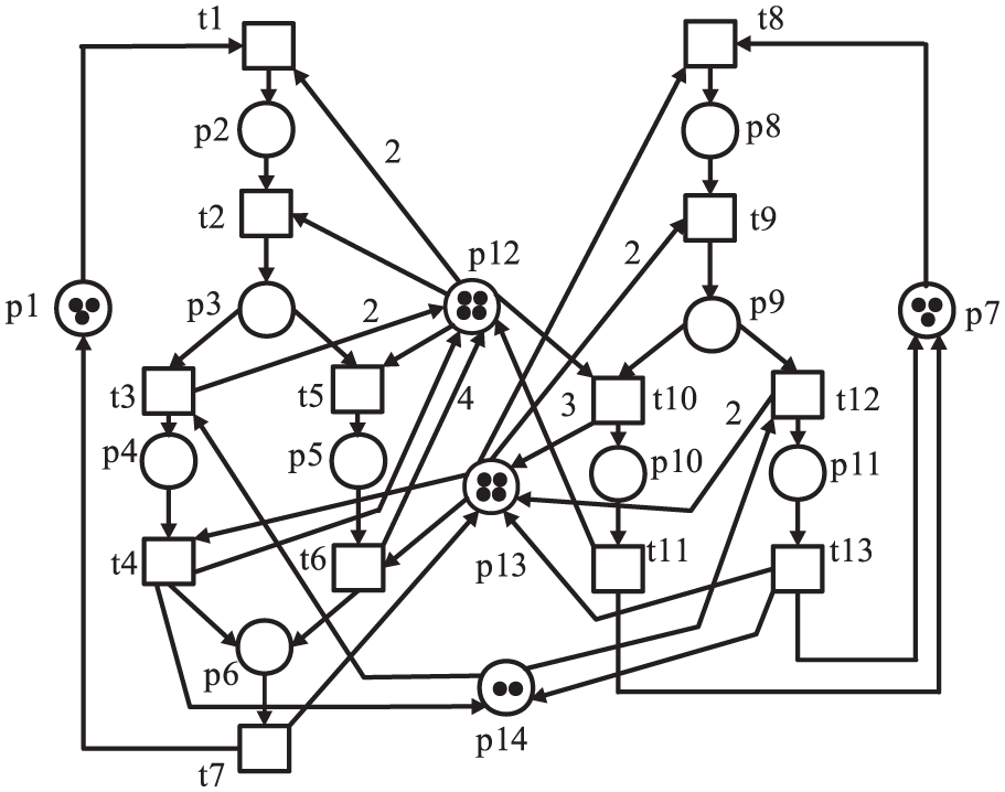
Figure 5 shows the non-live marked S⁴R, taken from Li et al., ²⁹ where $P^0=\{p_1,p_7\},P_A=\{p_2-p_6,p_8-p_{11}\},P_R=\{p_{12}-p_{14}\}$ , $|P|=|P^0|+|P_A|+|P_R|=14$ , and $|T|=13$ . Tables 7 and 8 show the control performance of the corresponding liveness-enforcing supervisors for $\mathrm{LL},\mathrm{UZ},\mathrm{and}\mathrm{PR}$ and the ICP comparison of different liveness-enforcing supervisors among $\mathrm{LL},\mathrm{UZ},\mathrm{and}\mathrm{PR}$ , respectively.

Figure 5.

A non-live marked S⁴R.

Table 7.

Control performance of the corresponding liveness-enforcing supervisors for $\mathrm{LL},\mathrm{UZ},\mathrm{and}\mathrm{PR}$ .

Item	Number of added CPs	Number of reachable states	${{}^{•}V}_k$	${V_k}^{•}$	$M_0(V_k)$
LL	3	312	$\{t_3,2t_4,4t_6,3t_{10},3t_{12}\}$	$\{2t_1,t_2,t_5,t_8,2t_9\}$	7
			$\{2t_2\}$	$\{2t_1\}$	2
			$\{t_9\}$	$\{t_8\}$	2
PR	3	85	$\{3t_3,t_4,4t_6,t_{11}\}$	$\{4t_1,t_{10}\}$	4
			$\{t_7,3t_{10},2t_{12},t_{13}\}$	$\{t_1,3t_8\}$	4
			$\{t_4,t_{13}\}$	$\{t_3,t_{12}\}$	2
UZ	3	322	$\{t_2\}$	$\{t_1\}$	1
			$\{t_9\}$	$\{t_8\}$	2
			$\{t_2,t_4,t_{10},t_{12}\}$	$\{t_1,t_3,t_8\}$	4

Table 8.

ICP comparison among liveness-enforcing supervisors for $\mathrm{LL},\mathrm{UZ},\mathrm{and}\mathrm{PR}$ .

Criteria	LL	PR	UZ
Variable region of $f_1$	[0, 5.20]	[0, 3.60]	[0, 2.99]
Variable region of $f_2$	[0, 6.18]	[0, 4.81]	[0, 4.63]
Satisfactory level $\lambda$	0.60	0.83	0.44
Optimal compromise solution of $f_1$ ( $f_1^{*}$ )	1.64	0.40	1.29
Optimal compromise solution of $f_2$ ( $f_2^{*}$ )	2.46	1.19	1.60
Qualitative evaluation	B	A	C

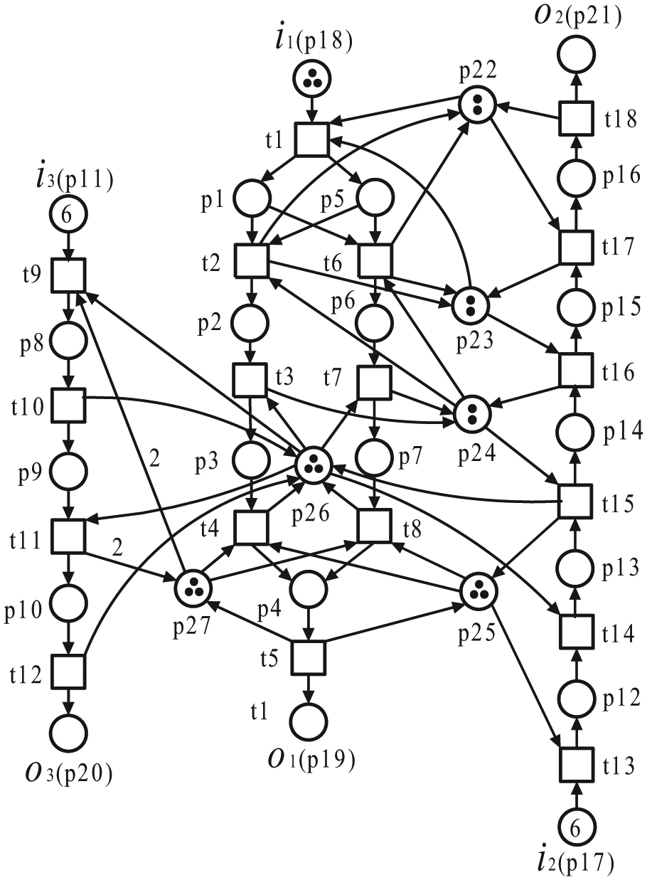
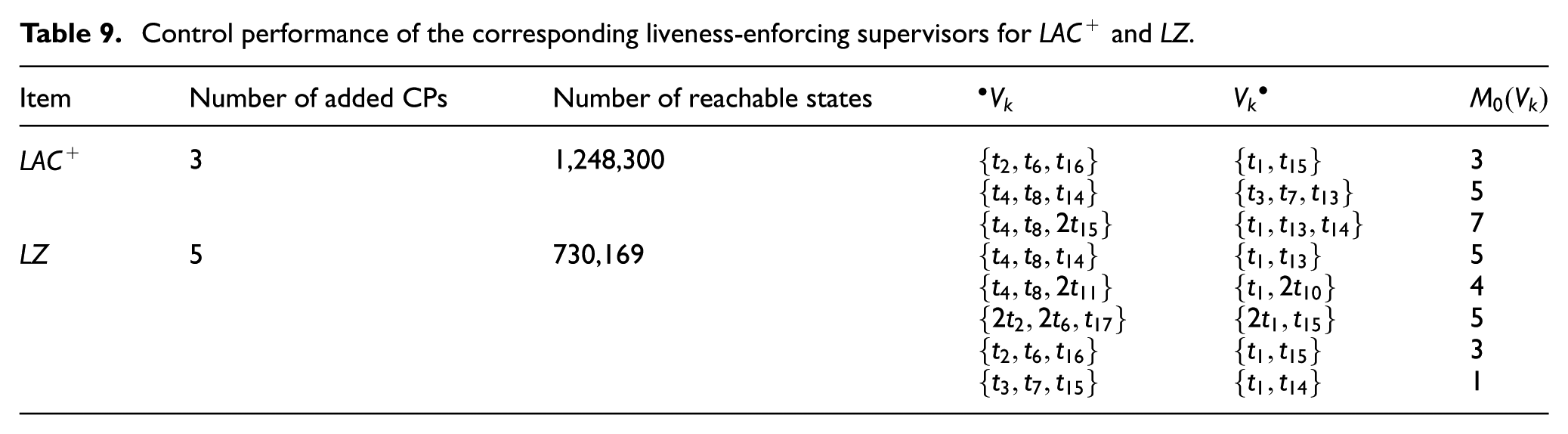
Finally, Figure 6 shows the non-live marked G-system, ²⁹ where $P_i=\{p_{11},p_{17},p_{18}\},P_o=\{p_{19}-p_{21}\},P_A=\{p_1-p_{10},p_{12}-p_{16}\},P_R=\{p_{22}-p_{27}\}$ , $|P|=|P_i|+|P_o|+|P_A|+|P_R|=27$ , and $|T|=18$ . Tables 9 and 10 show the control performance of the corresponding liveness-enforcing supervisors for $\mathrm{LA}{C}^{+}$ and LZ and the ICP comparison of different liveness-enforcing supervisors among $\mathrm{LA}{C}^{+}$ and LZ, respectively.

Figure 6.

A non-live marked G-system.

Table 9.

Control performance of the corresponding liveness-enforcing supervisors for $\mathrm{LA}{C}^{+}$ and LZ.

Item	Number of added CPs	Number of reachable states	${{}^{•}V}_k$	${V_k}^{•}$	$M_0(V_k)$
$\mathrm{LA}{C}^{+}$	3	1,248,300	$\{t_2,t_6,t_{16}\}$	$\{t_1,t_{15}\}$	3
			$\{t_4,t_8,t_{14}\}$	$\{t_3,t_7,t_{13}\}$	5
			$\{t_4,t_8,2t_{15}\}$	$\{t_1,t_{13},t_{14}\}$	7
LZ	5	730,169	$\{t_4,t_8,t_{14}\}$	$\{t_1,t_{13}\}$	5
			$\{t_4,t_8,2t_{11}\}$	$\{t_1,2t_{10}\}$	4
			$\{2t_2,2t_6,t_{17}\}$	$\{2t_1,t_{15}\}$	5
			$\{t_2,t_6,t_{16}\}$	$\{t_1,t_{15}\}$	3
			$\{t_3,t_7,t_{15}\}$	$\{t_1,t_{14}\}$	1

Table 10.

ICP comparison among liveness-enforcing supervisors for $\mathrm{LA}{C}^{+}$ and LZ.

Criteria	$\mathrm{LA}{C}^{+}$	LZ
Variable region of $f_1$	[0.33, 5.54]	[0.06, 4.25]
Variable region of $f_2$	[0, 1.07]	[0, 4.89]
Satisfactory level $\lambda$	0.67	0.59
Optimal compromise solution of $f_1$ ( $f_1^{*}$ )	1.80	1.79
Optimal compromise solution of $f_2$ ( $f_2^{*}$ )	3.50	2.02
Qualitative evaluation	B	B

From Tables 2, 4, 6, 8, and 10, it is shown how the ICP of different liveness-enforcing supervisors constructed by SBM or RGBM in the existing literature is. Moreover, the qualitative evaluations of the ICP for different liveness-enforcing supervisors can be given by means of a comparison of the values of $\lambda ,f_1^{*},\mathrm{and}{f}_2^{*}$ , which may give a referential guide for the determination of a liveness-enforcing supervisor among different ones.

Conclusion

Aiming at a problem on how to evaluate the ICP of liveness-enforcing supervisors in the existing literature, this research presents a novel algorithm to achieve the desired goal. Since the ICP evaluation problem for a liveness-enforcing supervisor involves several factors associated with the added CPs and the related input and output transitions,^1,2,39 two parameters $f_1$ and $f_2$ concerning with the number and initial markings for the added CPs, firing times (occurrences) of input and output transitions and the number and weight values of input and output control arcs are first introduced and then an MOLPP focusing on $f_1$ and $f_2$ and an LPP with $\lambda$ are designed, respectively, and embedded into the proposed Algorithm 1. For different liveness-enforcing supervisors constructed by SBM or RGBM, Algorithm 1 executes through two stages and finally yields the values of satisfactory level coefficients $\lambda$ and the optimal compromise solutions $f_1^{*}$ and $f_2^{*}$ of these liveness-enforcing supervisors. By means of a comparison of the values of $\lambda ,f_1^{*},\mathrm{and}{f}_2^{*}$ , the qualitative evaluations of the ICP for different liveness-enforcing supervisors can be given, which plays a positive role in selecting different liveness-enforcing supervisors designed by SBM or RGBM and enriches the related theory of evaluating a liveness-enforcing supervisor in terms of BP, SC, CC to some degree.