Sage Journals: Discover world-class research

Abstract

Aimed at studying the casing wear in the highly deviated well drilling, the experimental study on the casing wear was carried out in the first place. According to the test data and the linear wear model based on the energy dissipation proposed by White and Dawson, the tool joint–casing wear coefficient was obtained. The finite element model for casing wear mechanism research was established using ABAQUS. The nodal movement of the contact surface was employed to simulate the evolution of the wear depth, exploiting the Umeshmotion user subroutine. In addition, the time-dependent geometry of the contact surfaces between the tool joint and casing was being updated continuously. Consequently, the contact area and contact pressure were changed continuously during the casing wear process, which gives a more realistic simulation. Based on the shapes of worn casing, the numerical simulation research was carried out to determine the remaining collapse strength. Then the change curve of the maximum casing wear depth with time was obtained. Besides, the relationship between the maximum wear depth and remaining collapse strength was established to predict the maximum wear depth and the remaining strength of the casing after a period of accumulative wear, providing a theoretical basis for the safety assessment of worn casing.

Keywords

Experimental study casing wear user subroutine finite element collapse strength

Introduction

With the development of petroleum industry, extended-reach well, highly deviated well, ultra-deep well, and horizontal well technologies are widely applied in oil and gas drilling.^1–3 The highly deviated well in this article refers to the well with deviation angle greater than 45°.^4,5 Because of long drilling cycle, large friction, and big side force acting on the casing, the casing wear phenomenon is very severe. In addition, the remaining collapse resistance of the casing decreases drastically, even causing casing collapse phenomenon. As a result, it leads to a partial or full well abandonment and brings great inconvenience for the drilling operation and its subsequent completion and production.^6–8 In China, typical casing wear wells include Shengke-1, Yingke-1, Chegu-204, Dongqiu-5, Yacheng 13-1-3, and other dozens of wells.^8,9

Scholars have explored and proposed many research methods on the casing wear through experimental tests, numerical simulations, and field data. Through extensive experimental tests, Williamson¹⁰ proposed that a main factor affecting the casing wear was the magnitude of the loading between the joint and the casing and found an experimental relationship between the contact pressure and casing wear rate based on the new test machine. From the view of energy transfer and dissipation, White and Dawson¹¹ deduced the calculation method of the casing wear and developed the linear “wear efficiency” model to predict the casing wear. Song¹² studied the formula of the casing wear and presented an accurate method to calculate the strength of worn wear based on a crescent-shaped groove by building polar coordinate. Hall et al.¹³ argued that the casing wear is mainly associated with the wear coefficient, contact pressure, and sliding distance and deduced a prediction casing wear model based on the simplified static wear efficiency model. Gao and Sun¹⁴ modified the wear efficiency model by considering the change in the contact pressure during casing wear process and developed the nonlinear relationship of the wear depth and time. Through a wide variety of wells with measured depths (MDs) greater than 13,000 ft, Mitchell and Xiang¹⁵ created an extensive database and presented an improved casing wear prediction model using the statistically based model. Through the comparisons of different experimental tests, Sun et al.³ established a nonlinear wear model to consider running-in casing wear and steady-state casing wear during pipe rotation. Shen and Beck¹⁶ proposed an analytical solution for the stress evolution in worn casing based on the boundary superposition principle. Finite element solutions verified that the worn casing suffered from the expected stress concentration around the worn part. Wang et al.¹ established a three-dimensional (3D) finite element model to simulate the failure of the casing with uniform and non-uniform worn defects. Through the numerical simulations, the effects of worn defect type, defect length, wear percentage, drill string diameter, and casing wall thickness on the ultimate residual strength were studied systematically. Lin et al.¹⁷ established a new crescent-shaped wear equation for calculation of worn casing collapse strength considering both non-uniform wear and manufacturing defects. The equation had been successfully applied to casing design in oilfield and provided excellent effects.

As the time-dependent geometry of the contact surfaces between drill string and casing changes constantly and nonlinearly during casing wear process, it becomes too complex to accurately obtain contact pressure and sliding distance. Investigations found that previous researches generally adopted the “average contact” method to assume the contact pressure and total sliding distance in a period of wear.^{2,7,14,16–21} However, according to energy principle, the casing wear is a dynamic accumulation process, and the direct contact area between drill string and casing increases continuously and nonlinearly with the running wear. The maximum contact pressure of the drill string acting on the casing decreases with the increasing contact area. Therefore, the widely used average contact assumption is not appropriate and reasonable. In addition, the numerical simulation is a quicker and cheaper tool than the experimental test to predict evolution of the casing wear.

In order to improve this situation, casing tests were conducted in this study first, including friction and wear experiments. Then this article proposed a new method based on the numerical simulation. According to the redeveloped user subroutine—Umeshmotion—data interaction and parallel iterative computation between finite element software ABAQUS and FORTRAN programming were implemented to simulate the process of the casing wear. Finally, the remaining collapse strength was calculated based on the accumulative worn casing, using the ABAQUS restart function.

Experimental study

Friction coefficient experiment

Friction coefficient experiment was conducted in this article to obtain the average friction coefficient of P110 casing and tool joint. The testing machine was mainly composed of spindle driving system, fixture, load sensor, friction moment measurement system, loading system, and control panel, as shown in Figure 1.

Figure 1.

Friction testing machine.

The experimental specimens are shown in Figure 2. The ring was made from P110 casing, with outer diameter of 54 mm and inner diameter of 38 mm. The pin was made from the tool joint, with diameter of 4.7 mm.

Figure 2.

Experimental specimens.

In the experiment, when the rotating speed was constant, the normal load between the casing and tool joint specimens was changed and friction moment was measured. Friction coefficient can be expressed as

μ = \frac{M}{F \times r_{M}}

(1)

After processing the experimental data, the average friction coefficient of P110 casing and tool joint is 0.2087, as shown in Figure 3.

Figure 3.

Friction coefficient between tool joint and P110 casing.

Casing wear experiment

The wear coefficient has a significant effect on the prediction of the casing wear. In this study, casing wear experiment was carried out under different working conditions. There were two purposes to conduct the casing wear experimental tests. First, to obtain appropriate and accurate estimates of casing wear coefficient for the input to the numerical simulation, and second, to obtain worn shapes and volumes for validation of the numerically predicted results, as described later in section “Validation of the casing wear simulation—simulation under the experimental conditions.”

According to the linear model based on the energy dissipation proposed by White and Dawson,¹¹ the friction work done by friction between the drill pipe and casing can be expressed as

W = μ F_{N} L_{S}

(2)

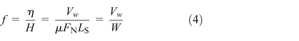
A portion of friction work is transformed into heat energy, and the other portion is manifested as the casing wear. The casing wear efficiency η can be calculated as

η = \frac{U}{W} = \frac{V_{w} H}{μ F_{N} L_{S}}

(3)

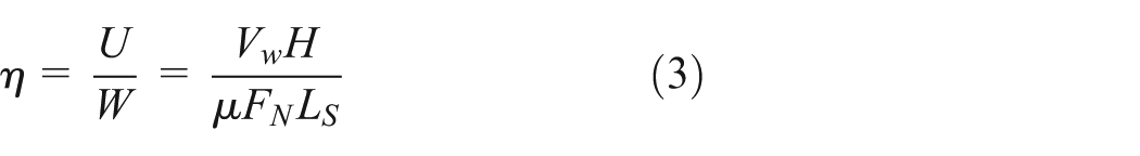
The wear coefficient f is as equation (4) according to equations (2) and (3)

f = \frac{η}{H} = \frac{V_{w}}{μ F_{N} L_{S}} = \frac{V_{w}}{W}

(4)

L_{S} = nt

(5)

According to equation (4), the casing wear coefficient can be calculated if the tests measure the casing wear volume under different rotating speeds and contact forces, as well as the wear time. The device for wear tests in this article is shown in Figure 4. In this experiment, the motor drove the tool joint specimen at a rotating speed of ω and the dead weight W was transferred to the constant load F_N applied on the casing specimen through load arm. Then the time-varying wear of the casing specimen (wear volume) can be obtained, as illustrated in Figure 5.

Figure 4.

Casing wear tester.

Figure 5.

Schematic diagram of wear tester.

The test materials were initially machined to specimens. The outer diameter of tool joint specimen S135 is 168 mm, and the width is 5 mm, as shown in Figure 6(a). The width of P110 casing specimen is 13 mm, as shown in Figure 6(b). In tests, the anti-high-temperature KCl drilling fluid with density of 1.02 g/cm³ was adopted. The experiment was conducted at contact force F_N from 60 to 120 N and the rotating speed of 60 r/min. After wear, both observation and measurement indicated that the morphology of the worn area on the casing specimen was typically crescent-shaped groove (as shown in Figure 7), which accorded with previous researches.¹

Figure 6.

Test sample of (a) tool joint and (b) casing.

Figure 7.

Morphology of worn area on casing specimen at different times: (a) 2 h, (b) 6 h, (c) 12 h, and (d) 20 h.

With the test data of equation (4) and Table 1, the wear coefficient curve of P110 casing and S135 tool joint in the anti-high-temperature KCl drilling fluid is calculated and shown in Figure 8. The curve presents a plot of the wear volume (V_w) as a function of the friction work (W) and confirms the linear relation with a good correlation (R² = 0.9865). Through the research,^7,11,22 wear coefficient is a parameter whose value ranges from 1.5 × 10⁻⁷ to 7.5 × 10⁻⁷ MPa⁻¹, which mainly depends on the mud type, properties, and solids’ content. In this article, the wear coefficient is 4.4566 × 10⁻⁷ MPa⁻¹, within the value ranges in the literatures. The obtained wear coefficient f is then implemented in the numerical model.

Table 1.

Test conditions and results.

Rotating speed (r/min)	Contact force (N)	Wear time (h)	Loss volume of wear (cm³)	Friction work (J) × 10⁷
60	60	2	0.0186	0.004758
60	60	4	0.0318	0.009516
60	60	6	0.0545	0.014275
60	60	10	0.0976	0.023792
60	60	12	0.1174	0.028550
60	60	14	0.1395	0.033309
60	60	20	0.2078	0.047584
60	90	2	0.0293	0.007137
60	90	4	0.0585	0.014275
60	90	6	0.0889	0.021413
60	90	10	0.1478	0.035688
60	90	12	0.1836	0.042826
60	90	14	0.2247	0.049963
60	90	20	0.3429	0.071376
60	120	2	0.0372	0.009516
60	120	4	0.0653	0.019033
60	120	6	0.1007	0.028550
60	120	10	0.1848	0.047584
60	120	12	0.2217	0.057101
60	120	14	0.2668	0.066618
60	120	20	0.4157	0.095168

Figure 8.

Wear coefficient between tool joint and P110 casing.

Numerical model of casing wear

Methodology of casing wear modeling

According to equation (5), it is worth noting that the casing wear is a complex and dynamic process, characterized by a time-varying load, a non-uniform contact pressure. So the casing wear is a time-dependent process. In such a case, equation (5) is rewritten and the wear depth on point M at instant time t can be expressed as follows

h (M) = f \int_{L_{M}} p (M, s) ds

(6)

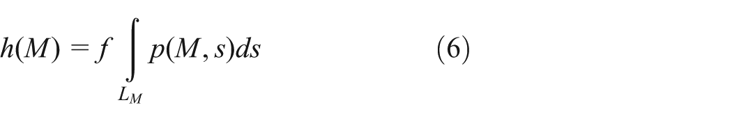
where s is the sliding distance along the traveled path L_M at t; p(M, s) is the instantaneous contact pressure in M at s.

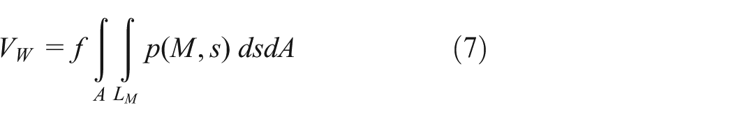
It is worth observing that the wear depth of each point at instant time t is different on the contact surface of the casing inner wall, because of the different instantaneous contact pressures and sliding distances that depend on the time. Thus, the volume loss of the casing can be obtained as

V_{W} = f \int_{A} \int_{L_{M}} p (M, s) dsdA

(7)

To numerically simulate the transient process of the casing wear, a large number N of cycles are established and each cycle can be treated as the static infinitesimal problem. Because of the ablation of the casing during the wear process, the contact pressure and sliding distance changed continuously. Therefore, it is essential to set up enough cycles to obtain a more realistic wear model. Then the dynamic process of the casing wear can be broken down into three basic procedures, including (1) solution of the contact problem to calculate the contact pressure and the sliding distance, (2) computation of the casing wear to calculate the wear depth and the volume loss, and (3) evolution and modification of contact surface geometry to build the new contact relationship. Each wear cycle i (i = 1, 2, 3,…, n) is performed, repeating the three procedures listed above. Hence, n geometry updates are performed to describe the dynamic process of the casing wear. The incremental wear depth $Δ h_{i}^{M}$ of ith cycle at point M can be expressed as

Δ h_{i}^{M} = {fp}_{i}^{M} (s_{i}^{M} - s_{i - 1}^{M})

(8)

where $s_{i}^{M}$ is the total tangential displacement of ith cycle at point M; $p_{i}^{M}$ is the contact pressure of ith cycle at point M.

Thus, the cumulative wear depth of the casing at point M is

h_{n}^{M} = \sum_{i = 1}^{n} Δ h_{i}^{M}

(9)

It should be noted that the wear depth increment is intended to lie along the normal to the surface, so a vector sum for all the casing wear surface is

h_{n}^{k} = \sum_{i = 1}^{n} Δ h_{i}^{k} n_{i}^{k}

(10)

where k is an arbitrary point of the contact surface; $n_{i}^{k}$ is the unit vector.

The methodology and the concept above are applied in the finite element modeling (FEM), and more specific implementation of FEM is described and illustrated in sections “Casing wear implementation of numerical simulation” and “Mesh and ALE adaptive meshing.”

Establishment of finite element model

The assumptions and simplifications were first made to the FEM as follows:

The problem is simplified as a two-dimensional (2D) plane problem focusing on the most serious location of wear along casing string.

The cross section of the casing is an absolute circle before wear and the casing material is the isotropic elastoplastic material.

The tool joint instead of drill pipe body contacts the inner wall of the casing.

The tool joint is assumed as a rigid body because the hardness of the tool joint is much higher than the casing.

The tool joint rotates on the casing inner wall with uniform speed and drill string vibration and buckling deformation are neglected.

The basic Coulomb friction model with isotropic friction is employed to simulate the casing wear.

In highly deviated wells, the position relationship of the tool joint and casing is shown in Figure 9. Because the outer diameter of the tool joint is larger than the drill string itself, the tool joint will first contact the inner wall of the casing and its high-speed rotating will cause the casing wear. Due to the well deviation, the tool joint contacts the casing inner wall and produces side contact force F_N on it. With the side contact force F_N, the tool joint causes the casing wear of different degrees within the contact area during the drill string rotating. From the geometric structure and force condition of the tool joint and casing in Figure 9, the wear process of the tool joint and casing can be simplified to a finite element mechanical model of 2D plane strain, as shown in Figure 10.

Figure 9.

Contact state of drill string and casing.

Figure 10.

FE model for tool joint–casing wear.

This article studied the tool joint with the outer diameter of 168 mm and the casing with steel grade of P110, outer diameter of 244.5 mm, and thickness of 11.05 mm. The casing was assumed as elastic–plastic deformable material. The mechanical properties of the casing material were as follows: density of 7580 kg/m³, Young’s modulus of 210 GPa, and Poisson’s ratio of 0.3. The engineering stress–strain curve of the casing is shown in Figure 11. It can be seen that the yield strength of P110 casing is 758.5 MPa. That is to say that the P110 casing will enter the yield phase when stress reaches 758.5 MPa, and the casing will be damaged and collapsed soon. The plastic behavior is modeled in ABAQUS by entering tabular data and interpolating material data will be implemented during analysis.

Figure 11.

Engineering stress–strain curve of P110 casing.

The hardness of the tool joint is far larger than that of the casing material, and the research object in this article is the P110 casing. Therefore, the tool joint was assumed as the analytical rigid body, which only had the functions of transferring the contact loads, rotating, wearing casing, and without producing deformation. The finite element model for tool joint–casing wear is shown in Figure 10.

Boundaries and initial conditions

Due to the cement fixation of the casing in the formation, the external boundaries of the casing in three directions are all constrained in the finite element model, as shown in Figure 10. The central reference point of the tool joint is RP1, which controls the constraints, load, and motion of the tool joint. The initial position of RP1 will be determined when the tool joint is in correct contact with the inner wall of the unworn casing at point C. In the process of the casing wear, the tool joint can only move along the y-axis and rotates around RP1. The RP1 is constrained in the x-direction and can move up and down in the y-direction. The load of RP1 is F_N. The z-axis translation degrees of freedom (DOFs) of tool joint are constrained, but the rotating DOF is not constrained. The rotating speed of the drill string around the z-axis is ω. The surface-to-surface interaction method and finite sliding contact approach were employed for the contact surface. The contact properties of the tool joint and casing wall are set, respectively, as follows: normal contact is set as hard contact; the Coulomb friction model with isotropic friction is applied to define the tangential behavior and the tangential contact friction coefficient is set as 0.2087.

Casing wear implementation of numerical simulation

According to the method and procedure described in section “Methodology of casing wear modeling,” in this section the casing wear implementation of the numerical simulation was based on these strategies. To simulate the dynamic process of the casing wear accurately, this article redeveloped user subroutine—Umeshmotion with FORTRAN programming language—to simulate the casing surface wear through the movement of the contact nodes. Umeshmotion is a user subroutine that can be used to define the motion of the nodes in an adaptive mesh constraint node area, and it provides interfaces to interact data with FORTRAN programming language.²³ The FE model of the casing wear provides a time-dependent geometry of the contact surfaces, which gives a more realistic simulation of the contact pressure and sliding distance. The concept of FEM is presented in Figure 12.

Figure 12.

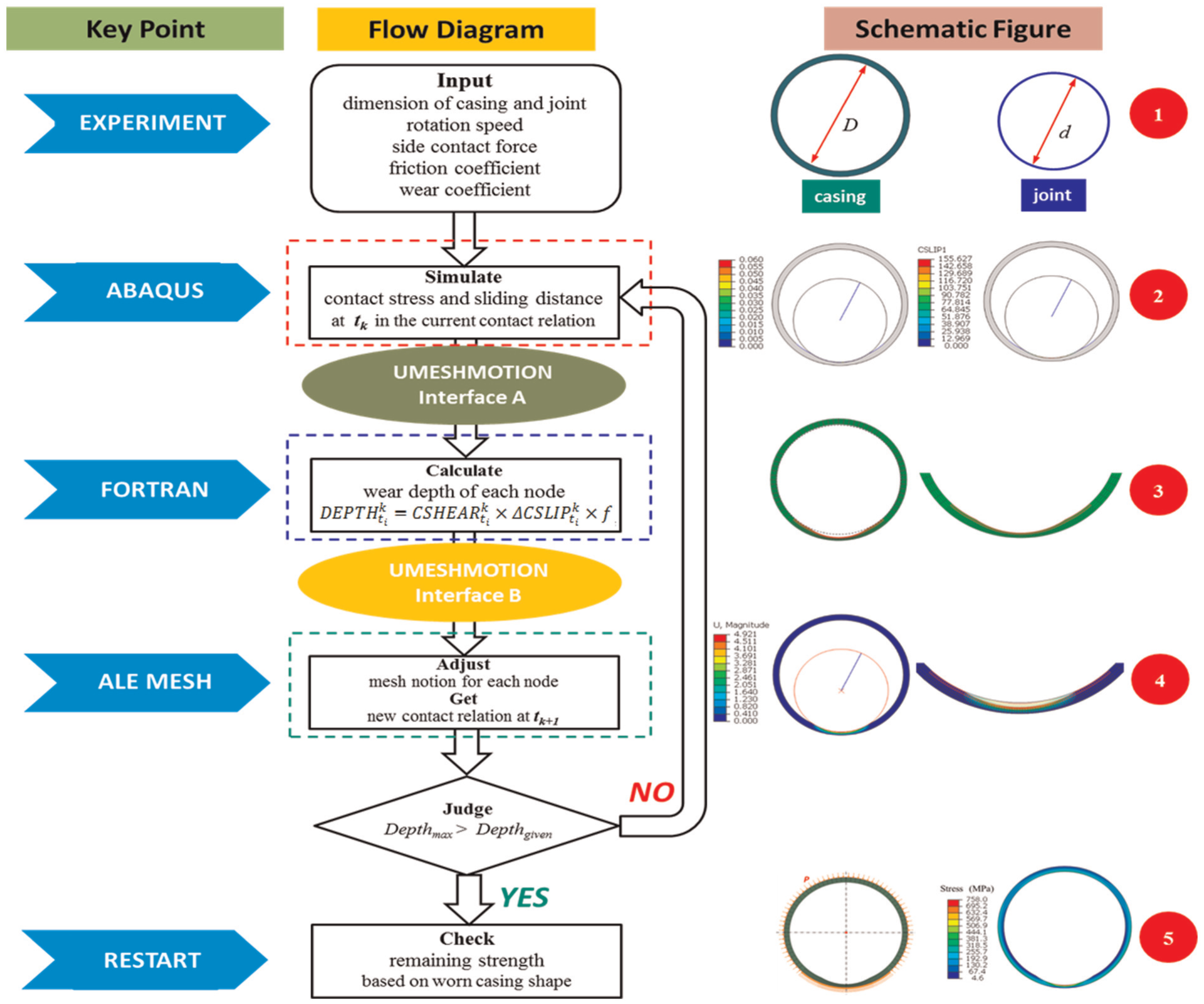
Schematic diagram of numerical simulation.

There were two steps built to simulate and solve the problem of the casing wear, including “initial contact step” and “wear process step.” In the first step, the initial problem of FE model was solved based on the material model, original mesh, contact geometry, and boundary conditions. Thus, the static infinitesimal contact problem between the casing and joint was simulated. Afterward, it is followed by the second step called wear process step, which is the key to solve the problem of the casing wear. In this step, the real contact area changed and consequently the contact pressure also changed. Hence, it is essential to consider enough increment numbers to obtain a more realistic wear model. One million increments were built, and the step time was divided into very small intervals. As the three basic procedures illustrated in section “Methodology of casing wear modeling,” first, the contact problem to calculate the contact pressure and the sliding distance was solved through ABAQUS standard FE solver. Then ABAQUS accessed the contact nodes one by one and recorded the properties for each node. The recorded nodal contact pressure and sliding distance were transferred from ABAQUS to FORTRAN programming through Umeshmotion interface A. Knowing the wear coefficient, contact pressure and sliding distance lead to the calculation of the wear depth. The wear depth of kth node at t_i was calculated in FORTRAN, according to equation (11)

{DEPTH}_{t_{i}}^{k} = {CSHEAR}_{t_{i}}^{k} \times Δ {CSLIP}_{t_{i}}^{k} \times f

(11)

where ${DEPTH}_{t_{i}}^{k}$ is the wear depth of kth node at t_i (mm), ${CSHEAR}_{t_{i}}^{k}$ is the shear stress of kth node at t_i (MPa), ${CSLIP}_{t_{i}}^{k}$ is the node sliding distance of kth node at t_i (mm), and f is the wear coefficient (MPa⁻¹).

Each node had its own local coordinate system ULOCAL and direction matrix ALOCAL in the global coordinate system, and the displacement vector of kth node at t_i in the global coordinate can be expressed as

{WGLOBA}_{t_{i}}^{k} = {ULOCAL}_{t_{i}}^{k} \times {ALOCAL}_{t_{i}}^{k}

(12)

Finally, the displacement data of each node were transferred back to ABAQUS through interface B. Once the above process was accomplished for all contact nodes, the nodes were swept in the normal direction and the worn boundary was remapped from the old position to the new position. This phase of remeshing geometry was performed via the arbitrary Lagrange–Euler (ALE) adaptive meshing, as described in section “Mesh and ALE adaptive meshing.” One cycle of casing wear process in the FE model was done, and an increment of wear evolution was implemented. After this, the new contact relationship at t_k+₁ was built and another round of iteration was executed to repeat the procedures above. The iteration process stopped when the maximum wear depth of the casing was greater than the given value. The ABAQUS restart function *Restart²³ was employed to calculate the remaining collapse strength based on the shape of worn casing.

Mesh and ALE adaptive meshing

Four-node plane strain CPE4 element type was selected for the casing. For the tool joint that was analytical rigid body, there was no need to be meshed. For the contact area of the casing, the mesh (element size) was very fine to capture the complicated variation in the contact pressure and sliding distance accurately. It is essential to achieve the correct balance between the accuracy and low computational cost for mesh refinement, which is discussed at the end of this section in detail.

In the simulation of a casing wear process, the nodal movement of the contact surface was employed to simulate the evolution of the wear depth. From Figure 13(b), the initial contact nodes (black points) were moved to the position of red nodes. However, if only the contact nodes are moved and proximity nodes are still in the original position, the mesh elements will be distorted and limited by the size and aspect ratio of elements, as illustrated in Figure 13(b). Therefore, ALE adaptive meshing was employed to solve this problem, which was performed on not only the contact elements but also their proximity elements. ALE adaptive meshing can maintain a high-quality mesh under severe material deformation by allowing the mesh to move independently of the underlying material and maintains a topologically similar mesh throughout the analysis (i.e. elements are not created or destroyed). The remeshed elements by ALE adaptive meshing technique are shown in Figure 13(c). It is worth noting that the mesh is still structured very well after the remeshing has been performed for the elements in the vicinity of the contact area.

Figure 13.

Comparison of initial mesh elements and remeshed elements: (a) geometry model; (b) mesh model and (c) remesh smoothing model.

The partition sizes and the mesh densities were also chosen according to the sensitivity analyses of the casing wear model mesh, in order to guarantee accuracy of simulation and low computational cost. The convergence of the numerical simulation required the mesh sensitivity analysis, according to which the mesh element size is repeatedly halved until the numerical result remains almost unchanged. Finally, the total number of elements is about 560 and the comparison of the computed results after mesh refinement indicates that the calculation accuracy can be improved with the increasing mesh density but the influence is very little, as illustrated in Figure 14. Therefore, the mesh number is sufficient for this particular problem. According to the function “verify mesh,” an estimate of mesh quality is good, including shape factor, small face corner angle, and aspect ratio.

Figure 14.

Contour comparison of two mesh densities.

Analysis of the FE numerical simulation

Validation of the casing wear simulation—simulation under the experimental conditions

According to equations (4) and (5), when side contact force F_N, friction coefficient µ, and wear coefficient f are constant, wear volume V_w is a time-related function (independent from geometrical shape of the casing). Therefore, based on the above finite element model, validation of casing wear simulation was conducted under the experimental conditions described in Table 1. Figure 15 shows a comparison of wear volume between the numerical simulations and experimental tests at different wear times. It is worth noting that the numerical results have good agreement with the test results. The margin of error is less than 5% and the maximum error is only 4.38% when the wear time is 4 h. Therefore, the finite element model and the methodology in this article are proved to be accurate and effective.

Figure 15.

Comparison of test and numerical simulation.

Analysis on the relationship of maximum wear depth and time

Based on the finite element model of tool joint–casing wear established in this article, a field condition is analyzed when the rotating speed of the drill string is 60 r/min and side contact force is 25 kN/m; the relationship curve (see Figure 16) of the maximum wear depth changing with time can be acquired through extensive numerical simulations. The location of the maximum wear depth refers to point c of the casing inner wall in Figure 10, and the depth gradually becomes smaller from point c to b and d, like a “crescent shape.” Comparison with the wear experiment and previous researches^1,7,12 verifies that the morphology of worn area on the casing is indeed a typically crescent-shaped groove; meanwhile, it proves the reliability and accuracy of this numerical simulation.

Figure 16.

Curve of casing maximum wear depth with time.

From the maximum casing wear curve in Figure 16, it can be seen that when the wear time of the tool joint and casing is within 55 h (see curve OM in Figure 16), the wear rate decreases with time, and the maximum wear depth and wear time present obvious nonlinear variation; when the wear time is over 55 h (55–155 h) (see curve MN in Figure 16), the casing wear rate basically remains stable, and the maximum wear depth and wear time approximately present linear relationship. The explanation of this phenomenon is related to the contact pressure of the worn area at the early stage of wear. The contact area of the tool joint and casing wall is small, so the high contact pressure makes the casing wear fast, whereas the maximum contact pressure becomes smaller as the wear goes on, which makes the casing wear rate slower to a stable value. According to the curve results in Figure 16, the maximum wear depth and the casing remaining strength in certain period of cumulative wear can be predicted.

In order to analyze the shapes of the casing wear more intuitively and clearly, five casing wear shapes of 10, 30, 55, 80, and 100 h are extracted from the results of the finite element numerical simulation, as shown in Figure 17. From Figure 17(1) to (5), it is known that the maximum casing wear depth all occurs in point c, and the maximum depths are 1.277, 2.570, 3.875, 5.006, and 6.030 mm, respectively. On the contrary, the residual wall thicknesses of the casing are 9.773, 8.480, 7.175, 6.044, and 5.020 mm, respectively. That means when the cumulative time of the casing wear reaches 100 h, the maximum wear depth of the casing is 6.030 mm, the residual wall thickness is 5.020 mm, and the wear rate comes to 54.57%, as shown in Figure 17(5). The position of the maximum tool joint–casing wear depth occurred at point c in the contact central area, and the depth decreases from point c to both sides. Points b and d are the correct unworn critical points. Figure 17 shows that the wear shape presents as “crescent” near the area bcd. Also, Figure 17 offers a great deal of data in terms of the wear shapes.

Figure 17.

Contours of casing maximum wear depth in different times.

Analysis on the remaining collapse strength after casing wear

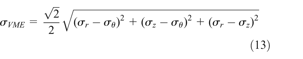
The reduction in the remaining collapse strength is significant and fast after casing wear; therefore, this article focuses on the analysis and study on the remaining collapse strength of worn casing. In the study, the ABAQUS restart function *Restart was used. On the basis of the shape after accumulative casing wear, the distributed pressure P was loaded on the surface of the outer diameter of casing to calculate the remaining collapse strength, as shown in Figure 18. According to the fourth strength theory (i.e. Von Mises criterion), the equivalent stress can be expressed as

σ_{VME} = \frac{\sqrt{2}}{2} \sqrt{{(σ_{r} - σ_{θ})}^{2} + {(σ_{z} - σ_{θ})}^{2} + {(σ_{r} - σ_{z})}^{2}}

(13)

Figure 18.

Restarted FE model for remaining collapse strength.

To ensure safety in casing strength design and evaluation, when σ_VME is greater than the yield strength of the casing material σ_s, the casing is considered as failure, and the distributed pressure P is fetched as the remaining collapse strength.^2,7–9,24

Figure 19 shows the contours of Von Mises stress when the first integration point of the casing just enters the yield phase ( $σ_{VME} = 758 MPa$ ). In Figure 19, the collapse loads of the casing before and after wear are P₁ and P₂, respectively. So P₁ and P₂ represent the collapse strength of the casing before and after wear, respectively. It is worth noting that when the casing is not worn, namely, the casing keeps perfect, the distribution of stress is uniform, and the collapse strength is P₁ = 29.96 MPa. The maximum stress of 758.0 MPa occurs on the inner wall of the casing uniformly. When the maximum wear depth of the casing is 3.875 mm, the remaining collapse strength is P₂ = 11.53 MPa. The Von Mises stress redistributes and is not uniform any more. The maximum stress of 758.1 MPa occurs on the area near the location of the maximum wear depth.

Figure 19.

Contours of Von Mises stress when casing just enters the yield phase: (a) no worn, wear depth = 0 mm and (b) 55 h, wear depth = 3.875 mm.

The relationship curve of the remaining collapse strength and maximum wear depth is created; the results are shown in Figure 20. It can be known from Figure 20 that the remaining collapse strength presents an approximately linear change with the maximum wear depth. It can be expressed as

P = - 4.4957 h_{w} + 30.518

(14)

where P is the remaining collapse strength (MPa); h_w is the maximum wear depth (mm).

Figure 20.

Curve of remaining collapse strength with maximum wear depth.

When the maximum wear depth of the casing is 0, the collapse strength is 29.96 MPa. When the maximum depth is 1.277 mm, the residual wall thickness of the casing is 9.773 mm, and the remaining collapse strength is 26.52 MPa. When the maximum depth is 2.570 mm, the residual wall thickness of the casing is 8.480 mm, and the remaining collapse strength is 18.93 MPa. When the maximum depth is 3.875 mm, the residual wall thickness of the casing is 7.175 mm, and the remaining collapse strength is 11.53 MPa. When the wear depth is more than half of the casing thickness and reaches 6.03 mm, the remaining collapse strength is only 5.02 MPa.

In order to verify the accuracy and reliability of the methods and results in this article, a comparison with the widely applied American Petroleum Institute (API)²⁵ formula is carried out. API formula is a series of experiment-based empirical equation to calculate collapse strength of worn casing. A uniform wear model is used in API formula; however, the casing wear between the tool joint and casing inner wall is a typical eccentric wear, as shown in Figure 21. Therefore, many scholars^8,9,18,26 point out that it is conservative and uneconomical to use API formula for the calculation and evaluation of the remaining strength of nonuniformly worn-out casing.

Figure 21.

Comparison of (a) eccentric wear and (b) uniform wear.

Compared with the calculation of API formula, it can be seen that casing strength results in API formula and numerical simulation are 30.78 and 29.96 MPa, respectively, when the casing is not worn, a difference of 2.75%. The numerical simulation accords with API standard, and the simulation result is slightly lower than API result, as shown in Figure 20. This indicates that the numerical simulation is consistent with and even safer than API standard in calculating the collapse strength of the casing with uniform thickness. However, when the casing is eccentrically worn, the difference between the numerical results and API results increases with the increase in the wear depth. When the casing is slightly worn, the numerical result is 15.06% higher than API result. When the wear depth is greater than a quarter of the casing thickness and smaller than half of the thickness, the difference is approximately 24%. Then the difference increases to 41.83% when the wear depth is more than half of the casing thickness and reaches 6.03 mm. API model assumes that the entire inner wall of the casing is uniformly worn and the wear area of API model is greater than the actual crescent-shaped wear, as shown in Figure 21. This difference will increase as the casing wear depth increases. So the error of the remaining strength between the value of API and numerical simulation increases gradually with the increase in the wear depth.

According to the comparison and analysis above, the numerical result accords with API standard and is slightly lower than API result for the casing with uniform thickness, which can also verify the accuracy and reliability of simulation method. When the casing is nonuniformly worn, however, it is conservative and uneconomical to use API formula for the calculation of the remaining strength because API formula assumes uniform casing wear rather than the actual crescent-shaped wear. This viewpoint also matches previous researches.^8,9,18,26 Based on the linear fitting formula (14) about the maximum wear depth and remaining collapse strength, the prediction and evaluation of worn casing remaining strength can be carried out with higher accuracy and reliability. The field application in several highly deviated wells in JD oilfield has verified the effectiveness and safety of the proposed prediction model.

Conclusion

Aiming at the highly deviated well drilling for oil and gas, this article proposed a complete system from the experimental tests, to the simulation of casing wear process, to the computation of the remaining strength. The conclusions can be drawn as follows:

Simulation under the experimental conditions and comparison of wear volume with experimental tests at different wear times validated the accuracy of FE model. Therefore, the relationship of the maximum casing wear depth changing with time was obtained, providing a real-time and dynamic prediction for casing wear process.

Based on the worn casing FE model, restart function was employed to simulate the collapse strength of the crescent-shaped wear casing. The linear fitting formula about the maximum wear depth and remaining collapse strength was obtained. Through the field application in JD oilfield of China, the effectiveness and safety of the prediction model have been verified.

Compared with the calculation of API formula, this article argues that it is reliable and safe to calculate casing strength of the uniform thickness; however, it is conservative and uneconomical to use API formula for the calculation and evaluation of the remaining strength of nonuniformly worn-out casing.

Footnotes

Appendix 1

Academic Editor: Noel Brunetiere

Declaration of conflicting interests

The author(s) declared no potential conflicts of interest with respect to the research, authorship, and/or publication of this article.

Funding

The author(s) disclosed receipt of the following financial support for the research, authorship, and/or publication of this article: The authors are grateful to the support from the National Natural Science Foundation of China (nos 51574198 and 51504207), Research Fund for the Doctoral Program of Higher Education of China (no. 20135121110005), and Key Project of Natural Science of Sichuan Education Department (no. 14ZA0037), for their contributions to this article.

References

Wang

Yan

Wang

. Investigation of the ultimate residual strengthen of a worn casing by using the arc-length algorithm. Eng Fail Anal 2013; 28: 1–15.

Gao

Sun

Lian

JH.

Prediction of casing wear in extended-reach drilling. Pet Sci 2010; 7: 494–501.

Sun

Gao

Zhu

Models & tests of casing wear in drilling for oil & gas. J Nat Gas Sci Eng 2012; 4: 44–47.

Wang

Mao

Han

. Directional well drilling technology. Beijing, China: Petroleum Industry Press, 2009.

Bai

YN.

Deviation control in directional drilling. Beijing, China: Petroleum Industry Press, 1990.

Lin

Shi

Research on casing wear mechanism and antiwear measures. Nat Gas Ind 2004; 7: 58–61 (in Chinese).

Liang

Han

. Analysis on collapse strength of casing wear. Chin J Mech Eng 2013; 26: 613–619 (in Chinese).

Liu

Zheng

Zhu

. Equations to calculate collapse strength of defective casing for steam injection wells. Eng Fail Anal 2014; 42: 241–251.

Zeng

Lin

Shi

New algorithm of collapsing strength of wearing casing. Nat Gas Ind 2005; 2: 78–80 (in Chinese).

10.

Williamson

JS.

Casing wear: the effect of contact pressure. J Petrol Technol 1981; 33: 2382–2388.

11.

White

Dawson

Casing wear: laboratory measurements and field predictions. SPE Drill Eng 1987; 2: 56–62.

12.

Song

JS.

The internal pressure capacity of crescent-shaped wear casing (SPE 23902). Richardson, TX: SPE, 1992.

13.

Hall

Jr Garkasi

Deskins

. Recent advances in casing wear technology (IADC/SPE 27532). Richardson, TX: SPE, 1994.

14.

Gao

Sun

LZ.

New method for predicting casing wear in horizontal drilling. Pet Sci Technol 2012; 30: 883–892.

15.

Mitchell

Xiang

Improving casing wear prediction and mitigation using statistically based model (SPE 151448). Richardson, TX: SPE, 2012.

16.

Shen

Beck

FE.

Intermediate casing collapse induced by casing wear in high-temperature and high-pressure wells (SPE 155973). Richardson, TX: SPE, 2012.

17.

Lin

Deng

Xing

. A new crescent-shaped wear equation for calculating collapse strength of worn casing under uniform loading. J Press Vess: T ASME 2015; 137: 031201.

18.

Liu

Xie

Liu

Research and application of casing wear prediction for extended reach well. Oil Drill Prod Technol 2010; 32: 11–15 (in Chinese).

19.

Lin

Deng

Sun

. Burst strength of tubing and casing based on twin shear unified strength theory. PLoS ONE 2014; 9: e111426.

20.

Texaco

Zhang

Casing burst strength after casing wear (SPE 94304). Richardson, TX: SPE, 2005.

21.

Wang

Research of friction and wear between drill pipe and casing. Qinhuangdao, China: Yanshan University, 2007 (in Chinese).

22.

Bradley

Fontenot

JE.

The prediction and control of casing wear. J Petrol Technol 1975; 27: 233–245.

23.

ABAQUS. ABAQUS documentation (Version 6.5). Providence, RI: Dassault Systemes Simulia Corp., 2005.

24.

Tan

Gao

Numerical analysis on the remaining collapsing strength of worn casing. Oil Drill Prod Technol 2000; 1: 6–8 (in Chinese).

25.

American Petroleum Institute (API). Bulletin on formulas and calculations for casing, tubing, drill pipe and line pipe properties (API bulletin 5C3). 6th ed. Washington, DC: API, 1994.

26.

Deng

Lin

Qiang

. New high collapse model to calculate collapse strength for casing. Eng Fail Anal 2015; 58: 295–306.

Experimental and numerical study on casing wear in highly deviated drilling for oil and gas

Abstract

Keywords

Introduction

Experimental study

Friction coefficient experiment

Casing wear experiment

Numerical model of casing wear

Methodology of casing wear modeling

Establishment of finite element model

Boundaries and initial conditions

Casing wear implementation of numerical simulation

Mesh and ALE adaptive meshing

Analysis of the FE numerical simulation

Validation of the casing wear simulation—simulation under the experimental conditions

Analysis on the relationship of maximum wear depth and time

Analysis on the remaining collapse strength after casing wear

Conclusion

Footnotes

Appendix 1

Declaration of conflicting interests

Funding

References