Sage Journals: Discover world-class research

Abstract

Signals in long-distance pipes are complex due to flow-induced noise generated in special structure, and the computation of these noise sources is difficult and time-consuming. To address this problem, a hybrid method based on computational fluid dynamics and Lighthill’s acoustic analogy theory is proposed to simulate flow-induced noise, with the results showing that the method is sufficient for noise predictions. The proposed method computes the turbulent flow field using detached eddy simulation and then calculates turbulence-generated sound using the finite element acoustic analogy method, which solves acoustic sources as volume sources. The velocity field obtained in the detached eddy simulation computation provides the sound source through interpolation between the computational fluid dynamics and acoustic meshes. The hybrid method is validated and assessed by comparing data from the cavity in pipe and large eddy simulation results. The peak value of flow-induced noise calculated at the monitor point is in good agreement with experimental data available in the literature.

Keywords

Pipes flow-induced noise computational fluid dynamics hybrid method detached eddy simulation

Introduction

As the analyzing of the signals in pipes is crucial for the safety monitoring, the prediction of these signal is studied in many experiments and numerical simulations.¹ For example, Moon et al.² used large eddy simulation (LES) to solve turbulent flows and obtained acoustic waves by solving the linearized perturbed compressible equations. The far field sound pressure of low subsonic turbulent flow noise predicted by their hybrid method was in excellent agreement with experimental measurements. Zhang et al.³ proposed a hybrid method that combined LES with Lighthill’s acoustic analogy to analyze the sound generated by turbulent flow passing through trash racks at the outlet of a pipeline, while Lee et al.⁴ computed the turbulent flow in a centrifugal blower and the resulting noise obtained from wall pressure fluctuations. Seo and colleagues^5,6 have proposed linearized perturbed compressible equations to compute low Mach number aeroacoustics.

Direct numerical simulation (DNS), LES, and the Reynolds-averaged Navier–Stokes method (RANS) are the three most commonly used methods in turbulence simulations, as can be seen in recent works.^7–10 Among these methods, DNS is too expensive in terms of computational resources, while RANS cannot provide accurate values for the pressure and velocity fluctuations that in turn determine the amplitudes of the sound sources. As a result, LES has become an important and widely used turbulence model for the simulation of flow-induced noise. However, LES theory dictates that this method needs a small size and high quality of boundary mesh. This is costly in terms of computation and memory although still much better than DNS in this regard.

Detached eddy simulation (DES) is a hybrid LES/RANS approach, first proposed by Spalart et al.,¹¹ which solves the flow near boundaries with RANS when the turbulent length scale is less than the product of a constant and grid size, otherwise solves the flow with LES. Thus, DES can considerably decrease computational costs, and a number of research works on DES methods have been published. Both RANS and DES were used to predict the flow around the Aerospatiale A-airfoil at maximum lift in Kotapati-Apparao et al.,¹² with preliminary DES predictions obtained based on experimental validated RANS results. Haupt et al.¹³ reported both DES and zonal DES results for flows through a surface-mounted cube at high Reynolds numbers. These two methods both produced high fidelity simulations with a modest grid resolution. Recently, zonal DES was used to investigate the unsteady separated flow around a leading-edge stall airfoil in post-stall conditions, with simulation results compared to detailed experimental results.¹⁴ A DES procedure was also given by Bozinoski and Davis¹⁵ to simulate the flow over a wall-mounted hump, and the mean attachment obtained by DES was in good agreement with experimental data from National Aeronautics and Space Administration (NASA). Details of this method were also provided in a recent review.¹⁶

Different DES methods have also been used to solve flow-induced noise problems. A novel DES, which used a monotone-integrated LES and RANS, was tested for jets in the case of co-flow, with the acoustics computed using the Ffowcs Williams and Hawkings method.¹⁷ In addition, Greschner et al.¹⁸ used a hybrid method combining DES based on a novel cubic explicit algebraic stress turbulence model with the Ffowcs Williams and Hawkings acoustic analogy method to predict sound generated by an airfoil in the wake of a rod.

The finite element acoustic analogy (FEAA) is a method based on Lighthill’s¹⁹ acoustic analogy theory that was first proposed by Oberai et al.,²⁰ and which is used in this article. This FEAA method has been used for aero^21,22 and hydro²³ flow-induced noise simulations, with some comparisons with experiments also available in the literature.^24–26 The approach relies on a variational formulation of Lighthill’s acoustic analogy, in which the acoustic analogy equations are discretized by a finite element discretization in Fourier space, which determines the radiated noise up to the free field, as introduced in Piellard and Coutty,²⁷ and Actran²⁸ and the instantaneous noise as in Caro et al.²⁹ Meanwhile, the method also solves the acoustic equations while taking into account the spectral volume and surface source.

This article is organized as follows. In section “Simulation strategy,” we build our hybrid method that combines DES and FEAA, providing both the basic theory and the simulation process. In section “Simulation strategy,” we establish the numerical model according to experimental models available in the literature. Section “Results and discussion” gives the numerical results obtained using our DES/FEAA hybrid method and compares the results against experimental data and results obtained using a LES/FEAA simulation. Finally, some conclusions and discussion of future work are given in section “Conclusion.”

Simulation strategy

Detached eddy simulation

DES is a method used to solve turbulent flows, and it combines RANS and LES methods. RANS is essentially applied to solve the boundary flow and LES is utilized to simulate the vortex. The turbulent model changes from RANS to LES when the turbulent length scale obtained by RANS is larger than the maximum grid dimension. The size requirement of the mesh near the solid boundary and the time step requirement are much lower when the boundary flow is solved by RANS than when it is determined by LES. As a result, the computational cost of RANS is lower than that of traditional LES-based methods.

The shear-stress transport (SST)-DES method³⁰ is applied to solve the boundary flow using the k-ω SST turbulent model. In this method, the governing equations are as follows

\frac{\partial (ρ k)}{\partial t} + u_{i} \frac{\partial (ρ k)}{\partial x_{i}} = P_{k} - ρ β^{*} k ω f_{β^{*}} + \frac{\partial}{\partial x_{i}} [(μ + \frac{μ_{t}}{σ_{k}}) \frac{\partial k}{\partial x_{i}}]

(1)

\begin{matrix} \frac{\partial (ρ ω)}{\partial t} + u_{i} \frac{\partial (ρ ω)}{\partial x_{i}} = P_{ω} - β_{ω} ρ ω^{2} \\ + \frac{\partial}{\partial x_{i}} [(μ + \frac{μ_{t}}{σ_{ω}}) \frac{\partial ω}{\partial x_{i}}] + 2 ρ (1 - F_{1}) \frac{1}{σ_{ω, 2} ω} \frac{\partial k}{\partial x_{j}} \frac{\partial ω}{\partial x_{j}} \end{matrix}

(2)

where ρ is the density, u_i is the velocity along the ith space coordinate, k is the turbulence kinetic energy, ω is the specific dissipation rate, P_k is the production term for k, µ is the dynamic viscosity, µ_t is the turbulent viscosity, and F₁ is the blending factor

P_{k} = \min (- τ_{ij} \frac{\partial u_{i}}{\partial x_{j}}, 10 ρ β^{*} k ω)

(3)

P_{ω} = \frac{α ω}{k} P_{k}

(4)

α = (\frac{β_{i, 1}}{β^{*}} - \frac{{0.41}^{2}}{σ_{ω, 1} \sqrt{β^{*}}}) F_{1} + (\frac{β_{i, 2}}{β^{*}} - \frac{{0.41}^{2}}{σ_{ω, 2} \sqrt{β^{*}}}) (1 - F_{1})

(5)

μ_{t} = \frac{ρ k}{\max (ω, \frac{S F_{2}}{a_{1}})}

(6)

F_{1} = \tanh {{\min [\max (\frac{\sqrt{k}}{β' ω d}, \frac{500 μ_{t}}{ρ ω d^{2}}) \frac{4 k ρ σ_{ω 2}}{d^{2} C D_{k ω}}]}^{4}}

(7)

F_{2} = \tanh {{[\max (\frac{2 \sqrt{k}}{0.09 ω d}, \frac{500 μ_{t}}{ρ ω d^{2}})]}^{2}}

(8)

C D_{k ω} = \max [2 ρ σ_{ω 2} \frac{1}{ω} (\frac{\partial k}{\partial x_{i}}) (\frac{\partial ω}{\partial x_{i}}), 10^{- 10}]

(9)

σ_{k} = \frac{1}{(F_{1} / σ_{k, 1}) + ((1 - F_{1}) / σ_{k, 2})}

(10)

σ_{ω} = \frac{1}{(F_{1} / σ_{ω, 1}) + ((1 - F_{1}) / σ_{ω, 2})}

(11)

β_{ω} = β_{i, 1} F_{1} + β_{i, 2} (1 - F_{1})

(12)

where τ_ij is the turbulent shear stress, S is the strain rate magnitude, and d is the distance to the surface. The following constants are used in our computation

\begin{matrix} β^{*} = 0.09, a_{1} = 0.31, σ_{k, 1} = 1.176, \\ σ_{ω, 1} = 2.0, σ_{k, 2} = 1.0, σ_{ω, 2} = 1.168, \\ β_{i, 1} = 0.075, β_{i, 2} = 0.0828 \end{matrix}

(13)

f_β* is defined as follows

f_{β^{*}} = \max (\frac{L_{t}}{C_{DES} Δ}, 1)

(14)

where C_DES is a calibration constant used in the DES model and has a value of 0.61, and Δ is the maximum local grid spacing. The turbulent length scale is the parameter that defines the RANS model

L_{t} = \frac{\sqrt{k}}{β^{*} ω}

(15)

Turbulent flow is solved with RANS when L_t is less than C_DESΔ. Otherwise, turbulent flow is solved with LES.

Finite element acoustic analogy

The FEAA method, as a novel implementation of Lighthill’s acoustic analogy, was first proposed by Oberai et al.²⁰ and further discussed in Oberai et al.³¹ and Caro et al.^29,32 The method is based on Lighthill’s equation

\frac{\partial^{2} ρ'}{\partial t^{2}} - c_{0}^{2} \frac{\partial^{2} ρ'}{\partial x_{i} \partial x_{i}} = \frac{\partial^{2} T_{ij}}{\partial x_{i} \partial x_{j}}

(16)

where $ρ'$ is the acoustic density, t is the time, and c₀ is the speed of sound at rest. Lighthill’s tensor T_ij is defined as follows

T_{ij} = ρ v_{i} v_{j} - τ_{ij} + δ_{ij} [(p - p_{0}) - c_{0}^{2} (ρ - ρ_{0})]

(17)

In resolving the above equation, we assume that the interaction between turbulent flow and sound can be disregarded. In the frequency domain, Lighthill’s equation can be obtained through harmonic expansion

- \frac{ω^{2}}{c_{0}^{2}} ψ - \frac{\partial^{2} ψ}{\partial x_{i} \partial x_{i}} = \frac{1}{i ω} \frac{\partial^{2} T_{ij}}{\partial x_{i} \partial x_{j}}

(18)

where

ψ = - \frac{ρ c_{0}^{2}}{i ω}

(19)

The strong variation statement associated with equation (3) can be written as follows

\int_{Ω} \frac{ω^{2}}{c_{0}^{2}} ψ δ ψ d Ω + \int_{Ω} \frac{\partial^{2} ψ}{\partial x_{i} \partial x_{i}} δ ψ d Ω = \int_{Ω} \frac{1}{i ω} \frac{\partial^{2} T_{ij}}{\partial x_{i} \partial x_{j}} δ ψ d Ω

(20)

where δψ is the test function, and Ω is the part of the computational domain. Spatial derivatives are integrated by parts in accordance with Green’s theorem to obtain a weak variational form

\begin{matrix} - \int_{Ω} \frac{ω^{2}}{ρ_{0} c_{0}^{2}} ψ δ ψ d Ω - \int_{Ω} \frac{1}{ρ_{0}} \frac{\partial ψ \partial δ ψ}{\partial x_{i} \partial x_{i}} d Ω \\ = \int_{Ω} \frac{i}{ρ_{0} ω} \frac{\partial δ ψ}{\partial x_{i}} \frac{\partial F (T_{ij})}{\partial x_{j}} d Ω - \int_{Γ} \frac{1}{ρ_{0}} F (ρ v_{i} n_{i}) d Γ \end{matrix}

(21)

where Γ is the surface of the computational domain.

In FEAA, Lighthill’s equation is modified using a finite element method (FEM) in the frequency domain. In this manner, dipoles are computed as a rigid wall boundary, and quadrupoles are simulated directly.

DES/FEAA hybrid method

The flow-induced noise simulation hybrid method in this article couples DES with the FEAA method. The main steps for performing the simulation are as follows:

Obtain the time history of unsteady velocity and pressure fluctuations through DES with the computational fluid dynamics (CFD) mesh during turbulent flow simulation;

Use the unsteady velocity and pressure field to compute the divergence of Lighthill’s tensor on the CFD mesh;

Map the calculated quantity onto the acoustic mesh by integrating over the CFD mesh with the shape functions of the acoustic mesh;³³

Transform the time-dependent data into the frequency domain using direct Fourier transform;

Perform the acoustic simulation with Lighthill’s acoustic analogy theory in the frequency domain (equation (6)).

Simulation strategy

Numerical model

For this article, we simulate a three-dimensional cavity model, which is similar to a valve, and which is similar to an experiment conducted by Lafon et al.³⁴ The inlet flow speed was U₀ = 62.8 m/s, which corresponds to a Mach number of 0.183. Characteristic dimensions of the model are shown in Figure 1: d = 0.05 m, h = 0.02 m, and L = 0.073 m. The air comes from the left of the figure and the vortex forms near the cavity. In the experiment, the cavity was installed in a wind tunnel whose height was 0.137 m. The width of the numerical model is 0.02 m. In the coordinate system, x points to the direction of outside flow and z points to the direction perpendicular to the bottom wall of cavity.

Figure 1.

Cavity model and its dimensions.

CFD mesh and boundary conditions

The CFD mesh and boundary conditions are shown in Figure 2. In the turbulent flow simulation, the inlet boundary is set as the velocity boundary, while the velocity profile is set the same as in the experiment. In addition, the outlet is the pressure boundary condition and the wall of the cavity is set as a no-slip wall. A structured mesh of 6.5 × 10⁵ is used in the DES computation, and the span of the simulation model is divided into 20 layers in the CFD mesh. The minimum grid size is 0.7 mm, and y⁺ is less than 100. The amount and grid size of the CFD mesh used in our study are almost the same as those used in a previous study to compare our findings with previously described numerical solutions.³ The time step in the LES computation is 8.0 × 10⁻⁵ s, so the Courant–Friedrichs–Lewy (CFL) number is between 1 and 5.

Figure 2.

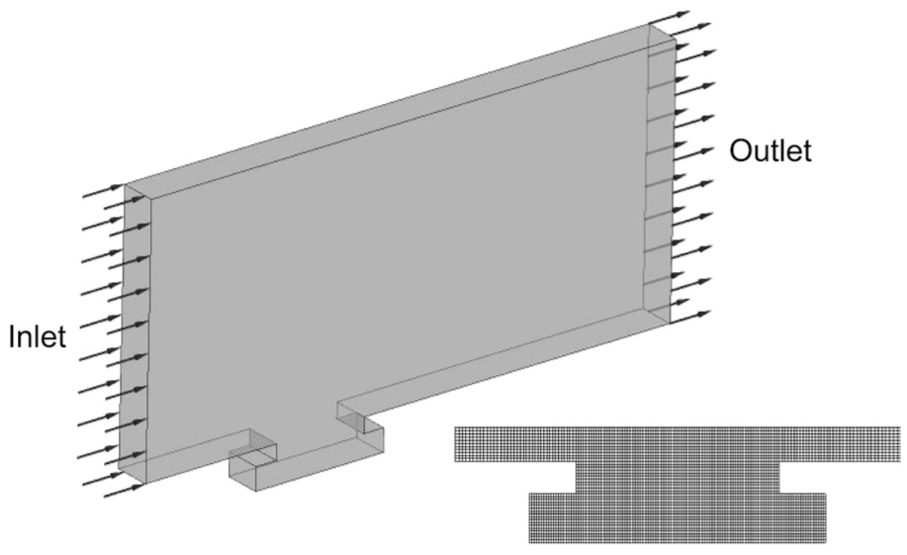
CFD mesh and boundary conditions.

Acoustic mesh and boundary conditions

The structured acoustic mesh and boundary conditions are shown in Figure 3. The FEAA computation uses two domains: the sound source domain and the sound propagation domain. The time history of velocity and pressure obtained from the LES computation are interpolated into the sound source domain. After the sound transforms through the sound propagation domain, it is computed by an infinite element method (IFEM).

Figure 3.

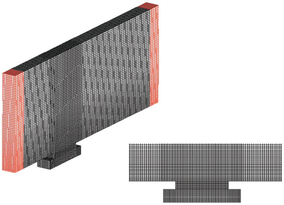
Acoustic mesh and boundary conditions.

The minimum grid size is 1 mm, resulting in a total of 1.8 × 105 elements. This mesh is compared with a coarse mesh and a fine mesh. The fine mesh contains approximately 2.7 × 10⁵ elements. The coarse mesh consists of approximately 9.0 × 10⁴ elements. The simulation results are shown in Figure 4. Figure 4 also reveals the sound pressure level (SPL) at a point 0.5 m above the bottom. Numerical results indicate that the three types of mesh slightly differ in the sound computation. Therefore, the level of the current mesh for acoustic analysis can be considered adequate. The wall of the sound source domain is assumed rigid while the wall of the sound propagation domain is set as the infinite acoustic boundary.

Figure 4.

SPL results of coarse mesh, computational mesh, and fine mesh at the observation point.

Results and discussion

Turbulent flow

The monitor point for the pressure is 0.1 m downstream from the center of the cavity. Figure 5 gives the time history of the pressure at the monitor point, with the time made dimensionless by multiplying by the maximum flow velocity and dividing by the length of the cavity. As can be seen from the figure, the pressure does change with time, but remains near a value of 2.0 × 10⁵ Pa and the range of the change is stable. Considering the properties of the LES model used in the DES method, this result shows that the CFD results are stable and thus can be used in our subsequent acoustic computation.

Figure 5.

Time history of the pressure fluctuations at the monitor point.

The two-dimensional cross-section velocity vectors for the region in and near the cavity are given in Figure 6. From the figure, we can see that the velocity of the flow inside the cavity is much lower than the outside flow. Moreover, a vortex generated by the outside flow occupies most parts of the cavity, and several small vortices form near the cavity wall. The flow velocity changes dramatically at the opening of the cavity, and the flow becomes unstable downstream.

Figure 6.

Velocity vector in and near the cavity.

Flow-induced noise

The SPL in the frequency domain at the monitor point located at the bottom center of the cavity is given in Figure 7, with the SPL from the monitor point 0.5 m away from the bottom also added to the figure for comparison.

Figure 7.

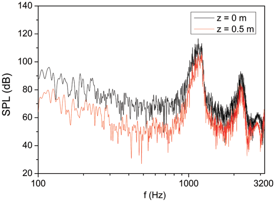
SPL of the monitor points 0 and 0.5 m from the bottom of the cavity.

For frequencies ranging from 100 to 3200 Hz, the SPL of the monitor point at the bottom of the cavity is larger than the SPL at a point 0.5 m above the bottom through virtually the entire measured frequency domain. Note that the SPL decreases with increasing frequency for frequencies lower than 500 Hz. Above this frequency, two peaks appear for both monitor points at approximately 1200 and 2300 Hz. We can explain this phenomenon using the excitation mode theory of the cavity, as described in the related experiment paper.³⁴ Furthermore, comparing Figure 7 and the results obtained in Zhang et al.,³ we can see that the peaks obtained by the DES/FEAA method are broader and less clear than the results obtained using the LES/FEAA method. The values for the frequency and SPL for both peaks corresponding to the monitor point at the bottom of the cavity are listed in Table 1.

Table 1.

Frequency and pressure level comparison between DES/FEAA and experiments.

	f₁ (Hz)	P₁ (dB)	f₂ (Hz)	P₂ (dB)
Exp	1199.5	124.3	2397.5	88.2
DES/FEAA	1156.6	116.8	2214.1	85.2
Error (%)	−3.6	−6.0	−7.6	−3.4
LES/FEAA³	1164.8	127.8	2329.8	95.5
Error (%)	−2.9	+2.8	−2.8	+8.3

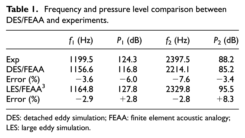
DES: detached eddy simulation; FEAA: finite element acoustic analogy; LES: large eddy simulation.

The experimental data³⁴ and the simulation results using the LES/FEAA method³ are also given in the table in order to validate our hybrid method. The percentage error values in Table 1 indicate the percent difference relative to the experimental data. In the simulation conducted by Lafon et al.,³⁴ the frequency of the first peak was in good agreement with the measured data although the pressure level was 17 dB lower than the experimental value. In addition, the second peak was not obvious. According to the table, the frequencies of the two peaks obtained through the DES/FEAA method are lower than the experimental data. Moreover, the results obtained by the LES/FEAA method are more accurate than the DES/FEAA hybrid method, particularly for predicting the first peak. However, it is worth noting that both methods obtain results that are acceptable for engineering applications.

Figure 8 shows the SPL contour of the mid-section at 500 and 1000 Hz. As shown in the figure, the noise source is mainly on the downstream side of the opening. The SPL at 1000 Hz inside the cavity is much higher than at 500 Hz, which shows the effects of the first peak.

Figure 8.

SPL contour at 500 and 1000 Hz.

Conclusion

We have developed a hybrid DES and FEAA method that simulates flow-induced noise at low Mach numbers in pipes. During simulation, the turbulent flow is computed using DES. Flow-induced sound is obtained through FEM based on Lighthill’s acoustic analogy theory. A three-dimensional cavity model is simulated. Our results are validated using experimental data from previous studies.

The DES computation effectively simulates the turbulent flow. The FEAA method also successfully predicts the acoustic field. Therefore, the feasibility of this hybrid method is confirmed. Furthermore, numerical results show less than 8% error in predicting SPL peak values at the test point. This finding indicates that the proposed DES/FEAA hybrid method is sufficiently accurate for use in engineering applications. The DES computation is also faster than the LES method. Our simulation further demonstrates that the noise source for the valve-equivalent model used in this article is near the opening of the cavity.

Footnotes

Academic Editor: Ramoshweu Lebelo

Declaration of conflicting interests

The author(s) declared no potential conflicts of interest with respect to the research, authorship, and/or publication of this article.

Funding

The author(s) disclosed receipt of the following financial support for the research, authorship, and/or publication of this article: This work was supported by Chongqing Key project of science and technology (Grant No. cstc2012gg-sfgc00002).

References

Wang

Freund

Lele

SK.

Computational prediction of flow-generated sound. Annu Rev Fluid Mech 2006; 38: 483–512.

Moon

Seo

Bae

. A hybrid prediction method for low-subsonic turbulent flow noise. Comput Fluids 2010; 39: 1125–1135.

Zhang

Ouyang

. Flow-induced noise analysis for 3D trash rack based on LES/Lighthill hybrid method. Appl Acoust 2014; 79: 141–152.

Lee

Jeong

. Numerical investigation on the characteristics of flow-induced noise in a centrifugal blower. Int J Fluid Mach Syst 2014; 7: 7–15.

Seo

Moon

YJ.

Linearized perturbed compressible equations for low Mach number aeroacoustics. J Comput Phys 2006; 218: 702–719.

Seo

Mittal

A high-order immersed boundary method for acoustic wave scattering and low-Mach number flow-induced sound in complex geometries. J Comput Phys 2011; 230: 1000–1019.

Wang

Sun

. Large-eddy/Reynolds-averaged Navier–Stokes simulation of combustion oscillations in a cavity-based supersonic combustor. Int J Hydrogen Energ 2013; 38: 5918–5927.

Xiao

Dianat

McGuirk

JJ.

Large eddy simulation of liquid-jet primary breakup in air crossflow. AIAA J 2013; 51: 2878–2893.

Wang

Shangguan

Onodera

. Direct numerical simulation and large eddy simulation on a turbulent wall-bounded flow using lattice Boltzmann method and multiple GPUs. Math Probl Eng 2014; 2014: 742432.

10.

Agarwal

RK.

Shape optimization of NREL S809 airfoil for wind turbine blades using a multiobjective genetic algorithm. Int J Aerosp Eng 2014; 2014: 864210.

11.

Spalart

Jou

Strelets

. Comments on the feasibility of LES for wings, and on a hybrid RANS/LES approach. In: Proceedings of the advances in DNS/LES: 1st AFOSR international conference on DNS/LES, Arlington, TX, 4–8 August 1997. Columbus, OH: Greyden Press.

12.

Kotapati-Apparao

Squires

Forsythe

. Prediction of the flow over an airfoil at maximum lift. In: Proceedings of the 42nd AIAA aerospace sciences meeting and exhibit, aerospace sciences meetings, Reno, NV, 5–8 January 2004, AIAA paper 2004-259, vol. 259. Reston, VA: AIAA.

13.

Haupt

Zajaczkowski

Peltier

LJ.

Detached eddy simulation of atmospheric flow about a surface mounted cube at high Reynolds number. J Fluid Eng: T ASME 2011; 133: 031002.

14.

Le Pape

Richez

Deck

. Zonal detached-eddy simulation of an airfoil in poststall condition. AIAA J 2013; 51: 1919–1931.

15.

Bozinoski

Davis

RL.

A DES procedure applied to a wall-mounted hump. Int J Aerosp Eng 2012; 2012: 149461.

16.

Spalart

PR.

Detached-eddy simulation. Annu Rev Fluid Mech 2009; 41: 181–202.

17.

Tucker

PG.

Novel MILES computations for jet flows and noise. Int J Heat Fluid Fl 2004; 25: 625–635.

18.

Greschner

Thiele

Jacob

. Prediction of sound generated by a rod–airfoil configuration using EASM DES and the generalised Lighthill/FW-H analogy. Comput Fluids 2008; 37: 402–413.

19.

Lighthill

Waves in fluids. Cambridge: Cambridge University Press, 2001.

20.

Oberai

Roknaldin

Hughes

TJR

. Computational procedures for determining structural-acoustic response due to hydrodynamic sources. Comput Method Appl M 2000; 190: 345–361.

21.

Caro

Ploumhans

Gallez

. A new CAA formulation based on Lighthill’s analogy applied to an idealized automotive HVAC blower using AcuSolve and Actran/LA. In: Proceedings of the AIAA/CEAS 11th aeroacoustics conference, Monterey, CA, 23–25 May 2005, pp.23–25. Reston, VA: AIAA.

22.

Liu

Zhang

YO.

Numerical study on flow-induced noise for a steam stop-valve using large eddy simulation. J Mar Sci Appl 2013; 12: 351–360.

23.

Zhang

Ouyang

Structural vibration and fluid-borne noise induced by turbulent flow through a 90° piping elbow with/without a guide vane. Int J Pres Ves Pip 2014; 125: 66–77.

24.

Zhang

TY.

Flow-induced noise simulation based on LES/Lighthill hybrid method. Appl Mech Mater 2014; 614: 428–431.

25.

Piellard

Bailly

. Several computational aeroacoustics solutions for the ducted diaphragm at low Mach number. In: Proceedings of the 16th AIAA/CEAS aeroacoustics conference, Stockholm, 8 June 2010. Reston, VA: AIAA.

26.

Piellard

A hybrid method for computational aeroacoustics applied to confined geometries. PhD Dissertation, Ecole centrale de Lyon, Ecully, 2008.

27.

Piellard

Coutty

. Application of a hybrid computational aeroacoustics method to an automotive blower. In: Proceedings of the vehicle concept modeling in the automotive sector workshop, Brussels, 6–7 June 2011. Woodhead Publishing Limited.

28.

Actran. Actran 11.1 user’s guide. Free Field Technologies, 2010.

29.

Caro

Ploumhans

Gallez

. Implementation of Lighthill’s acoustic analogy in a finite/infinite elements framework. In: Proceedings of the 10th AIAA/CEAS aeroacoustics conference, Manchester, 10–12 May 2004. Reston, VA: AIAA.

30.

Strelets

Detached eddy simulation of massively separated flows. Reston, VA: AIAA, 2001.

31.

Oberai

Roknaldin

Hughes

TJR

. Computation of trailing-edge noise due to turbulent flow over an airfoil. AIAA J 2002; 40: 2206–2216.

32.

Caro

Sandboge

Iyer

. Presentation of a CAA formulation based on Lighthill’s analogy for fan noise. In: Proceedings of the fan noise 2007 conference, Lyon, 17–19 September 2007, pp.17–19. Cetim.

33.

Carton de Wiart

Geuzaine

Detandt

. Validation of a hybrid CAA method: noise generated by a flap in a simplified HVAC duct. In: Proceedings of the 16th AIAA/CEAS aeroacoustics conference, Stockholm, 7–9 June 2010. Reston, VA: AIAA.

34.

Lafon

Caillaud

Devos

. Aeroacoustical coupling in a ducted shallow cavity and fluid/structure effects on a steam line. J Fluid Struct 2003; 18: 695–713.

Flow-induced noise simulation using detached eddy simulation and the finite element acoustic analogy method

Abstract

Keywords

Introduction

Simulation strategy

Detached eddy simulation

Finite element acoustic analogy

DES/FEAA hybrid method

Simulation strategy

Numerical model

CFD mesh and boundary conditions

Acoustic mesh and boundary conditions

Results and discussion

Turbulent flow

Flow-induced noise

Conclusion

Footnotes

Declaration of conflicting interests

Funding

References