Design of decentralized proportional–integral–derivative controller based on decoupler matrix for two-input/two-output process with active disturbance rejection structure

Abstract

The framework of the active disturbance rejection internal model control is proposed to solve the problem of the model reduced-order error in the process of the controller design for two-input/two-output system with time delay. In the controller design process of the two-input/two-output system, the decoupler matrix method is used to decompose a multi-loop control system into a set of equivalent independent single loops. Then, a complex equivalent model is obtained, and its order should be reduced for each individual loop. Maclaurin series method is used to reduce the order of the decoupling model. After reducing model order, the proposed method is applied to lessen the effect of the reduced-order error and improve the anti-interference ability and robustness for the control system. Simulation results show that the proposed method possesses a good disturbance rejection performance.

Introduction

Many chemical industrial processes can be described as the multivariable process. Due to the interactions between the input and output variables, the design process of the multivariable controller is complicated. To simplify the design procedure of the multivariable controller, a decoupler is designed to decompose a multi-loop control system into a set of equivalent independent single loops. Three types of basic decoupler design method are available: ideal, simplified, and inverted decoupling.

The two-input/two-output (TITO) process is the most common multivariable system in industry, such as continuous stirred tank reactor and chemical reactor. Many scholars concern on the design controller of the TITO with dead-time process.^1,2 Tong and Wang ³ addressed the problem of fuzzy robust decentralized control for a class of fuzzy large-scale systems with time delay based on the Takagi–Sugeno (T-S) fuzzy model and developed both fuzzy state feedback decentralized controller and fuzzy observer-based decentralized controller. Liu et al. ⁴ studied an adaptive neural output feedback tracking control of uncertain nonlinear multi-input–multi-output (MIMO) systems in the discrete-time form and developed an adaptive neural output feedback control for MIMO nonlinear discrete-time systems with the couplings in unknown functions. Li et al. ⁵ investigated the adaptive neural network (NN) control for a class of block triangular MIMO nonlinear discrete-time systems with each subsystem in pure-feedback form with unknown control directions and designed adaptive output NN controls for the nonlinear MIMO system based on the prediction control. Liu et al. ⁶ addressed the problems of stability and tracking control for a class of large-scale nonlinear systems with unmodeled dynamics by designing the decentralized adaptive fuzzy output feedback approach. Bhalodia and Weber ⁷ described a model for a TITO interacting process which characterizes the four open-loop responses by six time constants and two interacting gain factors; and then, proportional–integral (PI) controllers were applied to two feedback control loops. Lawrence and Douglas ⁸ detailed an applied investigation of pattern recognition based on adaptive control for TITO systems. Palmor et al. ⁹ presented a new algorithm for automatic tuning of decentralized proportional–integral–derivative (PID) control for TITO plants that fully extends the single-loop relay auto-tuner to the multi-loops case. Liu et al. ¹⁰ proposed a new analytical decoupling control scheme that was based on a standard internal model control (IMC) ¹¹ structure, which was capable of absolute decoupling regulation for the nominal binary system output responses. Li et al. ¹² designed a new identification method based on the decentralized step-test for TITO processes with significant interactions. Pontus and Tore ¹³ treated controller design and tuning for systems with two input signals and two output signals in the process industry and proposed a controller structure which consisted of a decoupler and a diagonal PID controller. Rao et al.^14,15 proposed a decentralized controller design based on the direct synthesis method for TITO processes in the Smith predictor configuration.

Recently, many decoupling methods are proposed to deal with the loop interaction. Jevtović and Mataušek ¹⁶ proposed a method for designing multivariable controller based on ideal decoupler and PID controller optimization under constraints on the robustness and sensitivity to measurement noise. Vu and Lee ¹⁷ proposed a new analytical method based on the direct synthesis approach for the design of a multi-loop PI controller to achieve the desired closed-loop response for MIMO processes with multiple time delays. Nie et al.^18,19 presented a single-iteration strategy for the design of a multi-loop PI controller to achieve the desired gain and phase margins for TITO processes. Vargas et al. ²⁰ concerned the stabilization of discrete-time TITO linear time-invariant (LTI) systems over communication channels.

This article aims to improve the disturbance rejection performance of decoupling control system for TITO processes with the dead-time process. A compound control structure is introduced into the controller design process of decoupler matrix. The proposed control scheme can handle the error of the reduced-order process. Meanwhile, the proposed method shows the trade-off between the performance and the robustness.

Diagonal decoupling control

The TITO system is one of the most prevalent categories of multivariable systems, because there are real processes of this nature or because a complex process has been decomposed into TITO process with non-negligible interactions between its inputs and outputs. Decentralized PID controllers with decoupler are most commonly preferred for TITO processes. ²¹ The traditional decoupling control system is shown in Figure 1.

Figure 1.

Control structure of decoupling control system for TITO system.

Decoupler matrix method ²² is used in the design process of decentralized PID controllers for TITO plant. The procedure of the decoupler matrix method is given. Let the TITO plant be as follows

$$G(s)=\left[\begin{array}{cc}{g}_{11}(s)e^{-{\tau }_{11}s}\hfill & g_{12}(s)e^{-{\tau }_{12}s}\hfill \\ \multicolumn{1}{c}{g_{21}(s)e^{-{\tau }_{21}s}}& g_{22}(s)e^{-{\tau }_{22}s}\hfill \end{array}\right]$$

(1)

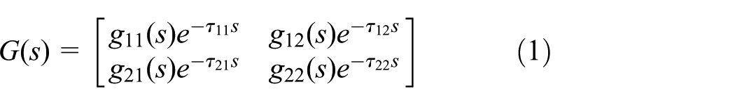
To design decoupler matrix, the following two cases are considered:

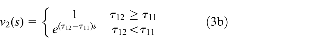
• Case 1. The off-diagonal elements of G(s) have no right-half-plane (RHP) poles and diagonal elements of G(s) have no RHP zeros. The decoupler matrix is

$$D(s)=\left[\begin{array}{cc}{v}_1(s)\hfill & d_{12}(s)v_2(s)\hfill \\ \multicolumn{1}{c}{d_{21}(s)v_1(s)}& v_2(s)\hfill \end{array}\right]$$

(2)

where

$$v_1(s)=\{\begin{array}{cc}1\hfill & {\tau }_{21}\ge {\tau }_{22}\hfill \\ \multicolumn{1}{c}{e^{({\tau }_{21}-{\tau }_{22})s}}& {\tau }_{21}<{\tau }_{22}\hfill \end{array}$$

(3a)

$$v_2(s)=\{\begin{array}{cc}1\hfill & {\tau }_{12}\ge {\tau }_{11}\hfill \\ \multicolumn{1}{c}{e^{({\tau }_{12}-{\tau }_{11})s}}& {\tau }_{12}<{\tau }_{11}\hfill \end{array}$$

(3b)

$$d_{12}(s)=-\frac{g_{12}(s)}{g_{11}(s)}{e}^{-({\tau }_{12}-{\tau }_{11})s}$$

(3c)

$$d_{21}(s)=-\frac{g_{12}(s)}{g_{11}(s)}{e}^{-({\tau }_{12}-{\tau }_{11})s}$$

(3d)

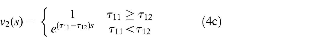
• Case 2. The diagonal elements have no RHP poles and off-diagonal elements have no RHP zeros of G(s). The decoupler matrix is

$$D(s)=\left[\begin{array}{cc}{d}_{11}(s)v_1(s)\hfill & v_1(s)\hfill \\ \multicolumn{1}{c}{v_2(s)}& d_{22}(s)v_2(s)\hfill \end{array}\right]$$

(4a)

where

$$v_1(s)=\{\begin{array}{cc}1\hfill & {\tau }_{22}\ge {\tau }_{21}\hfill \\ \multicolumn{1}{c}{e^{({\tau }_{22}-{\tau }_{21})s}}& {\tau }_{22}<{\tau }_{21}\hfill \end{array}$$

(4b)

$$v_2(s)=\{\begin{array}{cc}1\hfill & {\tau }_{11}\ge {\tau }_{12}\hfill \\ \multicolumn{1}{c}{e^{({\tau }_{11}-{\tau }_{12})s}}& {\tau }_{11}<{\tau }_{12}\hfill \end{array}$$

(4c)

$$d_{11}(s)=-\frac{g_{22}(s)}{g_{21}(s)}{e}^{-({\tau }_{22}-{\tau }_{21})s}$$

(4d)

$$d_{22}(s)=-\frac{g_{11}(s)}{g_{12}(s)}{e}^{-({\tau }_{11}-{\tau }_{12})s}$$

(4e)

As shown in equation (5), $\overline{G}(s)$ is a diagonal matrix

$$\overline{G}(s)=G(s)D(s)=\mathrm{diag}({\overline{g}}_{\mathrm{ii}}(s))=\left[\begin{array}{cc}{\overline{g}}_{11}(s)\hfill & 0\hfill \\ \multicolumn{1}{c}{0}& {\overline{g}}_{22}(s)\hfill \end{array}\right]$$

(5)

The decoupled elements ${\overline{g}}_{\mathrm{ii}}(s)$ , where i = 1,2, are to be controlled through decentralized PID controllers.

Model reduced-order method

The dynamics of the elements ${\overline{g}}_{\mathrm{ii}}(s)$ of $\overline{G}(s)$ are quite complex. Due to the complexity of the decoupled model, it cannot be applied to design of controller using the traditional design method. So, the high-order model should be reduced in order to design the controller. The frequency of the reduced model approximates that of the original model. However, the reduced model order affects the performance of the control system. So, the proposed method is applied to lessen the effect of the reduced-order error and improve the anti-interference ability and robustness for the control system.

A first-order plus dead-time (FOPDT) model often reasonably describes the process gain, overall time constant, and effective dead time of higher order processes. Thus, the model order is reduced to simplify the derivation for higher order processes. Many methods can be used to reduce order, such as polynomial approximation, ²³ the Gaussian frequency domain approach, ²⁴ and least squares algorithm. ²⁵ Model reduction can be described as searching a low-order model with a small time delay to approximate the full-order model. In this section, a simple Maclaurin series reduction-order method ²⁶ is shown. A FOPDT model ${\overline{g}}_{\mathrm{ii}}^r(s)$ of each element ${\overline{g}}_{\mathrm{ii}}(s)$ of $\overline{G}(s)$ is obtained as follows

$${\overline{g}}_{\mathrm{ii}}^r(s)=\frac{K_{\mathrm{ii}}{e}^{-{\theta }_{\mathrm{ii}}s}}{t_{\mathrm{ii}}s+1}$$

(6)

${\overline{g}}_{\mathrm{ii}}(s)$ is expanded in a Maclaurin series. The result is given by

$${\overline{g}}_{\mathrm{ii}}(s)=a_{\mathrm{ii}}+b_{\mathrm{ii}}s+c_{\mathrm{ii}}{s}^2+d_{\mathrm{ii}}{s}^3+e_{\mathrm{ii}}{s}^4+O(s^5)$$

(7)

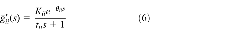
where the coefficients of equation (7) polynomial are

$$a_{\mathrm{ii}}={\overline{g}}_{\mathrm{ii}}(0)$$

(8a)

$$b_{\mathrm{ii}}=\frac{d{\overline{g}}_{\mathrm{ii}}(s)}{\mathrm{ds}}{|}_{s=0}$$

(8b)

$$c_{\mathrm{ii}}=\frac{1}{2}\frac{d^2{\overline{g}}_{\mathrm{ii}}(s)}{d{s}^2}{|}_{s=0}$$

(8c)

$$d_{\mathrm{ii}}=\frac{1}{6}\frac{d^3{\overline{g}}_{\mathrm{ii}}(s)}{d{s}^3}{|}_{s=0}$$

(8d)

$$e_{\mathrm{ii}}=\frac{1}{24}\frac{d^4{\overline{g}}_{\mathrm{ii}}(s)}{d{s}^4}{|}_{s=0}$$

(8e)

Expanding the reduced diagonal matrix, given by equation (6), into a Maclaurin series in s results in

$${\overline{g}}_{ii}^r(s)=K_{ii}-K_{ii}\left({\theta }_{ii}+t_{ii}\right)s+K_{ii}\left[\frac{1}{2}{\theta }_{ii}^2+\left({\theta }_{ii}+t_{ii}\right)t_{ii}\right]s^2+O_{ii}\left(s^3\right)$$

(9)

where K, t, and $\theta$ should be identified to approximate ${\overline{g}}_{\mathrm{ii}}(s)$ as close as possible over relevant frequency ranges. Trying the following: comparing the first, the second, and the third terms in equation (9) with those in equation (7) leads to the following explicit equations for K, t, and $\theta$

$$K_{\mathrm{ii}}=a_{\mathrm{ii}}$$

(10a)

$$t_{\mathrm{ii}}=\sqrt{\frac{2c_{\mathrm{ii}}}{a_{\mathrm{ii}}}-{\left(\frac{b_{\mathrm{ii}}}{a_{\mathrm{ii}}}\right)}^2}$$

(10b)

$${\theta }_{\mathrm{ii}}=-\frac{b_{\mathrm{ii}}}{a_{\mathrm{ii}}}-\sqrt{\frac{2c_{\mathrm{ii}}}{a_{\mathrm{ii}}}-{\left(\frac{b_{\mathrm{ii}}}{a_{\mathrm{ii}}}\right)}^2}$$

(10c)

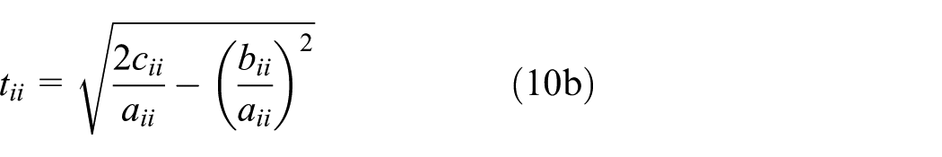
To get feasible results for the FOPDT model, t and $\theta$ should be real and positive. It is clear from equation (10) that the following condition should be satisfied for feasible t and $\theta$ values

$$\sqrt{\frac{2c_{\mathrm{ii}}}{a_{\mathrm{ii}}}}>(-\frac{b_{\mathrm{ii}}}{a_{\mathrm{ii}}})>\sqrt{\frac{2c_{\mathrm{ii}}}{a_{\mathrm{ii}}}-{\left(\frac{b_{\mathrm{ii}}}{a_{\mathrm{ii}}}\right)}^2}$$

(11)

Remark 1

Any technique can be applied toward fitting the decoupled model into a low-order model. In this work, for the purpose of evaluating the proposed method, a simple model reduced technique was adopted based on the coefficient matching method. Maclaurin series method is based on the coefficient matching method without considering the frequency response fitting; Maclaurin series method makes the readers understood easily; the obtained reduced error fits to demonstrate the property of the proposed method. So, Maclaurin series is applied into model reduced order in this article.

Active disturbance rejection control structure

A composite control structure is proposed to conquer the drawback of the reduced error and improve the system robustness. In other words, a design method of the active disturbance rejection internal model control (ADRIMC) is proposed. Then, the design procedures are shown.

Control structure

The system structure of ADRIMC is shown in Figure 2.

Figure 2.

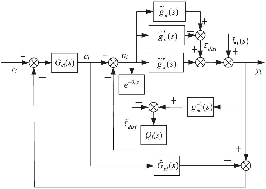
ADRIMC scheme for each loop.

In Figure 2, r_i(s) and y_i(s) define the reference input and output, respectively; τ_disi(s) and ξ_i(s) define the internal disturbance and the external disturbance, respectively; G_ci(s) defines the controller of ADRIMC controller; u_i and c_i define the external control law and the internal control law, respectively; and ${\hat{\tau }}_{\mathrm{disi}}$ defines the estimation disturbance.

Let

$${\overline{g}}_{\mathrm{ii}}^r(s)=g_{\mathrm{ni}}(s)e^{-{\theta }_{\mathrm{ni}}s}$$

(12)

Q(s) is low-pass filter (LPF), which is given by

$$Q(s)=\frac{1+\sum _{k=1}^{N-m}{a}_k{({\lambda }_{1i}s)}^k}{1+\sum _{k=1}^N{a}_k{({\lambda }_{1i}s)}^k}$$

(13)

where N is the order of Q(s), λ_1i is the filter time constant of the ith loop, and m is the relative degree of Q(s). ²⁷

In Figure 2, the transfer function of the output response is given by

$$y_i={\overline{g}}_{\mathrm{ii}}(s)u_i+D_i(s)$$

(14)

where the equivalent disturbance input is given by

$$D_i(s)={\xi }_i(s)+{\tau }_{\mathrm{disi}}(s)$$

(15)

Then, the estimate disturbance is given by

$${\hat{\tau }}_{\mathrm{disi}}(s)=Q_i(s)g_{\mathrm{ni}}^{-1}(s)y_i-Q_i(s)u_i{e}^{-{\theta }_{\mathrm{ni}}s}$$

(16)

From equations (14)–(16), it is known that the estimate disturbance can be defined as

$${\hat{\tau }}_{\mathrm{disi}}(s)=Q_i(s)g_{\mathrm{ni}}^{-1}(s)D_i(s)$$

(17)

In Figure 2, from the first summing point, we have

$$u_i=c_i-{\hat{\tau }}_{\mathrm{disi}}(s)$$

(18)

By substituting equation (17) into equation (18), the transfer function of the manipulate variable is obtained as

$$u_i=c_i-Q_i(s)g_{\mathrm{ni}}^{-1}(s)D_i(s)$$

(19)

Then, if the transfer function of the manipulate variable is known, according to equation (14), the transfer function of the output response is obtained as

$$y_i=c_i{\overline{g}}_{\mathrm{ii}}^r(s)+[1-Q_i(s)e^{-{\theta }_{\mathrm{ni}}s}]D_i(s)$$

(20)

Remark 2

Although the equivalent disturbance D_i(s) is unknown, the equivalent disturbance has a steady-state value, that is, satisfies $\underset{s\to 0}{lim}D(s)<\infty$ . The filter Q(s) in the ADRIMC satisfies $\underset{s\to 0}{lim}Q(s)=1$ . So, the following equation is established: $\underset{s\to 0}{lim}[1-Q_i(s)e^{-{\theta }_{\mathrm{ni}}s}]D_i(s)=0$ . The final transfer function is $\underset{s\to 0}{lim}{y}_i=\underset{s\to 0}{lim}{c}_i{\overline{g}}_{\mathrm{ii}}^r(s)$ .

Thus, when the equivalent disturbances have a steady-state value, the suitable ${\lambda }_{1i}$ is selected to conquer the disturbance influence.

Note that

$$G_{\mathrm{pi}}(s)={\overline{g}}_{\mathrm{ii}}^r(s)$$

(21)

$$G_{\mathrm{di}}(s)=1-Q_i(s)e^{-{\theta }_{\mathrm{ni}}s}$$

(22)

then, the transfer function of the output response can be described as

$$y_i=G_{\mathrm{pi}}(s)c_i+G_{\mathrm{di}}(s)D_i(s)$$

(23)

where G_pi(s) is the modified controlled plant model and G_di(s) is the disturbance filter.

Based on the above discussion, the system structure of ADRIMC is shown in Figure 3. Compared with the traditional IMC structure, a disturbance filter G_di(s) is located at the disturbance input in the ADRIMC structure. The disturbance filter can ensure that the ADRIMC scheme realizes the effectiveness of the ADR for the error of the reduced order. The internal model structure can ensure that the ADRIMC scheme realizes the effectiveness of the deviation-integration in itself.

Figure 3.

Equivalent block diagram for each loop.

Tuning controller parameters

The parameter ${\lambda }_1$ is tuned by the balance tuning technique. ²⁸ Assume that the controlled plant of the each loop is second-order plus dead-time (SOPDT) model, as shown in the following equation

$$G_{\mathrm{pi}}(s)=\frac{k_i}{{\tau }_{1i}{s}^2+{\tau }_{2i}s+1}{e}^{-{\theta }_{i}s},G_{p0i}(s)=\frac{k_i}{{\tau }_{1i}{s}^2+{\tau }_{2i}s+1}$$

(24)

And then, the IMC controller is obtained by the following equation

$$G_{Ci}(s)=\frac{{\tau }_{1i}{s}^2+{\tau }_{2i}s+1}{k_i}\frac{{\beta }_{i}s+1}{{({\lambda }_{1i}s+1)}^3}=\frac{({\beta }_{i}s+1)({\tau }_{1i}{s}^2+{\tau }_{2i}s+1)}{k_i{({\lambda }_{1i}s+1)}^3}$$

(25)

where ${\beta }_i={\alpha }_i{\lambda }_{1i}$ , ${\alpha }_i$ is the value of ${\beta }_i/{\lambda }_{1i}$ and ${\alpha }_i$ shows the filter characteristic.

The equivalent feedback controller $G_{0i}(s)$ is given by

$$G_{0i}(s)=\frac{G_{Ci}(s)}{1-G_{Ci}(s)G_i(s)}=\frac{({\beta }_{i}s+1)({\tau }_{1i}{s}^2+{\tau }_{2i}s+1)}{k_i{({\lambda }_{1i}s+1)}^3-k_i({\beta }_{i}s+1)e^{-{\theta }_{i}s}}$$

(26)

When $r_i(s)=1$ , $d_i(s)=0$ , and the model is matched, the closed-loop response of the system is shown in equation (27)

$$y_{\mathrm{ri}}(s)=\frac{G_{0i}(s)G_{\mathrm{pi}}(s)}{1+G_{0i}(s)G_{\mathrm{pi}}(s)}{r}_i(s)$$

(27)

When $r_i(s)=0$ , $d_i(s)=1$ , and the model is matched, the closed-loop response of the system is shown in equation (28)

$$y_{\mathrm{di}}(s)=\frac{G_{\mathrm{di}}(s)}{1+G_{0i}(s)G_{\mathrm{pi}}(s)}{D}_i(s)$$

(28)

where $y_{\mathrm{di}}(s)$ is the disturbance output of ith loop and $G_{0i}(s)$ is equivalent feedback controller of ith loop.

And then, the closed-loop response of the whole system is given by

$$y_i(s)=\frac{G_{0i}(s)G_{\mathrm{pi}}(s)}{1+G_{0i}(s)G_{\mathrm{pi}}(s)}{r}_i(s)+\frac{G_{\mathrm{di}}(s)}{1+G_{0i}(s)G_{\mathrm{pi}}(s)}{D}_i(s)$$

(29)

The input error of the control system is given by

$$e_{\mathrm{ri}}(s)=y_{\mathrm{ri}}(s)-r_i(s)=\frac{G_{0i}(s)G_{\mathrm{pi}}(s)}{1+G_{0i}(s)G_{\mathrm{pi}}(s)}{r}_i(s)-r_i(s)$$

(30)

The sensitivity function and the complementary sensitivity function are shown in equation (31)

$$S_i=\frac{1}{1+G_{0i}(s)G_{\mathrm{pi}}(s)},T_i=\frac{G_{0i}(s)G_{\mathrm{pi}}(s)}{1+G_{0i}(s)G_{\mathrm{pi}}(s)}$$

(31)

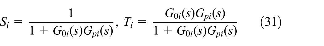
where $S_i{G}_{\mathrm{Ci}}(s)G_i(s)-1=T_i-1=-S_i$ .

Furthermore, the relationship between the input error and the sensitivity function is given by

$$e_{\mathrm{ri}}(s)=-S_i{r}_i(s)=(T_i-1)r_i(s)$$

(32)

According to equation (32), when the input sensitivity function is smaller and the complementary sensitivity function is larger, the system error is smaller. By substituting equation (27) into equation (31), the analytical expression of the sensitivity function is shown in equation (33)

$$S_i=\frac{1}{1+G_{0i}(s)G_{pi}(s)}=\frac{1}{1+\frac{({\beta }_{i}s+1)({\tau }_{1i}{s}^2+{\tau }_{2i}s+1)/k_i}{{({\lambda }_{1i}s+1)}^3-({\beta }_{i}s+1)e^{-{\theta }_{i}s}}{G}_{pi}(s)}$$

(33)

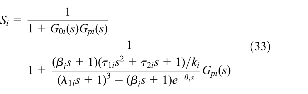
By simplifying equation (33), equation (34) can be obtained

$$S_i=1-\frac{({\beta }_{i}s+1)e^{-{\theta }_{i}s}}{{({\lambda }_{1i}s+1)}^3}$$

(34)

First-order Taylor approximation method is adopted to deal with the time delay part

$$e^{-{\theta }_{i}s}\approx 1-{\theta }_{i}s$$

(35)

By substituting equation (35) into equation (34), equation (36) can be obtained

$$S_i=\frac{{\lambda }_{1i}^3{s}^3+(3{\lambda }_{1i}^2-{\beta }_i{\theta }_i)s^2+(3{\lambda }_{1i}-{\beta }_i+{\theta }_i)s}{{\lambda }_{1i}^3{s}^3+3{\lambda }_{1i}^2{s}^2+3{\lambda }_{1i}s+1}$$

(36)

Let

$${\mu }_i=\frac{{\lambda }_{1i}}{{\theta }_i},{\gamma }_i=\frac{{\beta }_i}{{\theta }_i},s_i=\frac{{\eta }_i}{{\theta }_i}$$

(37)

where ${\gamma }_i/{\mu }_i={\beta }_i/{\lambda }_{1i}={\alpha }_i$ .

By substituting equation (37) into equation (36), the expression of the sensitivity function is obtained

$$S_i=\frac{{{\mu }_i}^3{{\eta }_i}^3+(3{{\mu }_i}^2-{\gamma }_i){{\eta }_i}^2+(3{\mu }_i-{\gamma }_i+1){\eta }_i}{{{\mu }_i}^3{{\eta }_i}^3+3{{\mu }_i}^2{{\eta }_i}^2+3{\mu }_i{\eta }_i+1}$$

(38)

The analytical expression of the maximum sensitivity function is shown in equation (39)

$$M_{\mathrm{si}}=\underset{0<\omega <\infty }{max}\left|\frac{{{\mu }_i}^3{{\eta }_i}^3+(3{{\mu }_i}^2-{\gamma }_i){{\eta }_i}^2+(3{\mu }_i-{\gamma }_i+1){\eta }_i}{{{\mu }_i}^3{{\eta }_i}^3+3{{\mu }_i}^2{{\eta }_i}^2+3{\mu }_i{\eta }_i+1}\right|$$

(39)

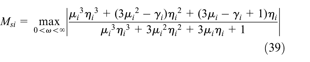
Based on ${\beta }_i=\alpha {\lambda }_{1i}$ , the relationship of $M_{\mathrm{si}}-{\mu }_i$ can be found, as shown in Figure 4. Where M_si is the maximum sensitivity function, and then the typical values of M_si are in the range of [1.0–2.0].

Figure 4.

Relationship of $M_{\mathrm{si}}-{\mu }_i$ .

Assuming that the system input of each loop is step response, integral absolute error (IAE) value from input to output is given by

$$\mathrm{IA}{\mathrm{E}}_{\mathrm{ri}}=\underset{0}{\overset{\infty }{\int }}|y_{\mathrm{ri}}(t)-r_i(t)|\mathrm{dt}$$

(40a)

$$\mathrm{IA}{\mathrm{E}}_{\mathrm{ri}}=\underset{0}{\overset{\infty }{\int }}\left|{\zeta }^{-1}\left(\frac{1}{s}(1-\frac{({\beta }_{i}s+1)e^{-{\theta }_{i}s}}{{({\lambda }_{1i}s+1)}^3})\right)\right|\mathrm{dt}$$

(40b)

The result is obtained by

$$\mathrm{IA}{\mathrm{E}}_{\mathrm{ri}}=\{\begin{array}{c}{t}_i\hfill \\ \multicolumn{1}{c}{3{\lambda }_{1i}-{\beta }_i+{\theta }_i}\end{array}\begin{array}{c}{t}_i\le \theta \hfill \\ \multicolumn{1}{c}{t_i>\theta }\end{array}$$

(41)

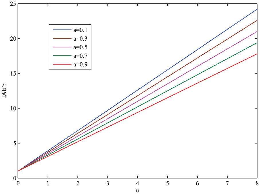
IAE value is manipulated by the scale transformation, as shown in equation (42)

$$\mathrm{IA}{\mathrm{E}\prime }_{\mathrm{ri}}=3{\mu }_i-{\gamma }_i+1$$

(42a)

$$\mathrm{IA}{\mathrm{E}\prime }_{\mathrm{ri}}=(3-{\alpha }_i){\mu }_i+1$$

(42b)

where $\mathrm{IA}{\mathrm{E}\prime }_{\mathrm{ri}}=\mathrm{IA}{\mathrm{E}}_i/{\theta }_i$ and ${\gamma }_i/{\mu }_i={\alpha }_i$ .

According to Figure 5, it is known that if $0<{\alpha }_i<3$ , then $min(\mathrm{IA}{\mathrm{E}\prime }_{\mathrm{ri}})=1$ ; if ${\alpha }_i>3$ , then $min(\mathrm{IA}E{\prime }_{\mathrm{ri}})=0$ and ${\mu }_i=1/{\alpha }_i-3$ . According to Figure 5, it is known that when ${\alpha }_i>3$ , the system robustness is bad. So, $0<{\alpha }_i<3$ is only considered, as shown in Figure 5.

Figure 5.

Relationship of $\mathrm{IA}{\mathrm{E}\prime }_{\mathrm{ri}}-{\mu }_i$ based on different $\alpha$ values.

It is known that balance tuning method is used for tuning the controller parameters ${\lambda }_{1i}$ by considering the robustness and stability. Furthermore, PID parameters of the controller are shown by

$$G_{0i}(s)=\frac{({\beta }_{i}s+1)({\tau }_{1i}{s}^2+{\tau }_{2i}s+1)}{k_i{({\lambda }_{1i}s+1)}^3-k_i({\beta }_{i}s+1)e^{-{\theta }_{i}s}}=\frac{1}{s}\overline{f_i}(s)$$

(43)

Then, expanding $C_i(s)$ in a Maclaurin series with s is given by

$${\mathrm{P}}_i(s)=\frac{\overline{f_i}(s)}{s}=\frac{1}{s}({\overline{f}}_i(0)+{\overline{f_i}}^{\prime }(0)s+\frac{{{\overline{f}}^{\prime \prime }}_i(0)}{2!}{s}^2+\cdots )$$

(44)

The corresponding PID expressions are given by

$$C_i(s)=K_{\mathrm{mi}}(1+\frac{1}{T_{\mathrm{Ii}}s}+T_{\mathrm{Di}}s)$$

(45)

$$\{\begin{array}{c}{K}_{\mathrm{Ci}}=\overline{f{\prime }_i}(0)\hfill \\ \multicolumn{1}{c}{T_{\mathrm{Ii}}=\frac{\overline{f{\prime }_i}(0)}{\overline{f_i}(0)}}\\ \multicolumn{1}{c}{T_{\mathrm{Di}}=\frac{\overline{f_i^{″}}(0)}{2\overline{f_i\prime }(0)}}\end{array}$$

(46)

The results are shown in equation (47)

$$\{\begin{array}{c}{K}_{\mathrm{Ci}}=\frac{(3{\lambda }_{1i}-{\beta }_i+{\theta }_i){\tau }_{2i}+3{\lambda }_{1i}^2-\frac{1}{2}{{\theta }_i}^2+{\beta }_i{\theta }_i}{k_i{(3{\lambda }_{1i}^2-{\beta }_i+{\theta }_i)}^2}\hfill \\ \multicolumn{1}{c}{T_{\mathrm{Ii}}=\frac{(3{\lambda }_{1i}-{\beta }_i+{\theta }_i){\tau }_{2i}+3{\lambda }_{1i}^2-\frac{1}{2}{{\theta }_i}^2+{\beta }_i{\theta }_i}{k_i(3{\lambda }_{1i}^2-{\beta }_i+{\theta }_i)}}\\ \multicolumn{1}{c}{T_D=\frac{k_i({\tau }_{2i}-{\tau }_{2i})(3{\lambda }_{1i}-{\beta }_i+{\theta }_i)-k_i{\tau }_{2i}(3{\lambda }_{1i}^2-\frac{1}{2}{{\theta }_i}^2+{\beta }_i{\theta }_i)+k_i[{\lambda }_{1i}^2-\frac{1}{6}(3{\beta }_i{{\theta }_i}^2-{{\theta }_i}^3)]}{-k_i(3{\lambda }_{1i}-{\beta }_i+{\theta }_i)+k_i(3{\lambda }_{1i}^2-\frac{1}{2}{{\theta }_i}^2+{\beta }_i{\theta }_i)}+T_{\mathrm{Ii}}}\end{array}$$

(47)

Similarly, the parameter ${\lambda }_{2i}$ can be tuned. The error between the disturbance and the output is given by

$$e_{\mathrm{di}}(s)=\frac{G_{\mathrm{di}}(s)}{1+G_{0i}(s)G_{\mathrm{pi}}(s)}{D}_i(s)-D_i(s)$$

(48)

When $\underset{s\to 0}{lim}{G}_{\mathrm{di}}(s)=0$ , the error between the disturbance and the output is maximum, and the disturbance rejection effective of the system is good.

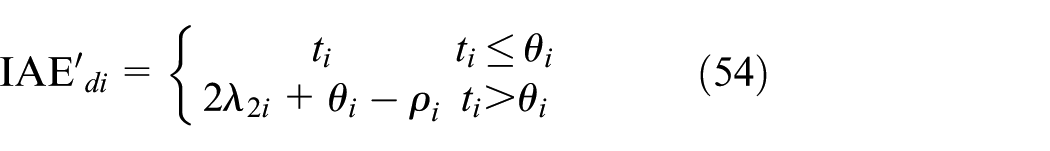
And then, calculation of the IAE value from the disturbance to the output is obtained by

$$\mathrm{IA}{\mathrm{E}}_{\mathrm{di}}=\underset{0}{\overset{\infty }{\int }}|y_{\mathrm{di}}(t)-d_i(t)|\mathrm{dt}$$

(49)

Assuming that the system input of each loop is step response

$$\mathrm{IA}{\mathrm{E}}_{\mathrm{di}}=\underset{0}{\overset{\infty }{\int }}\left|{\zeta }^{-1}\left\{\frac{1}{s}[\frac{G_{\mathrm{di}}(s)}{1+G_{0i}(s)G_{\mathrm{pi}}(s)}{D}_i(s)-D_i(s)]\right\}\right|\mathrm{dt}$$

(50)

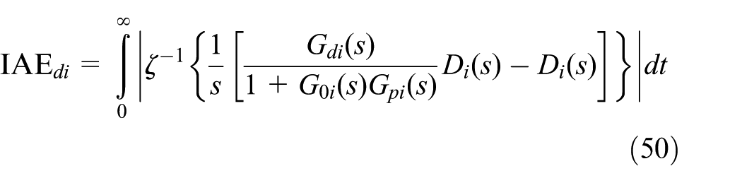
Let

$$\mathrm{IA}{\mathrm{E}\prime }_{\mathrm{di}}=\underset{0}{\overset{\infty }{\int }}\left|{\zeta }^{-1}[\frac{1}{s}(1-Q_i(s)e^{-{\theta }_{i}s})]\right|\mathrm{dt}$$

(51)

It can be seen from equation (51) that if $\mathrm{IA}{\mathrm{E}\prime }_{\mathrm{di}}\to 0$ , then $\mathrm{IA}{\mathrm{E}}_{\mathrm{di}}\to$ maximum (Figure 6). Assuming that

$$Q_i(s)=\frac{{\rho }_{i}s+1}{{({\lambda }_{2i}s+1)}^2}$$

(52)

where ${\rho }_i={\kappa }_i{\lambda }_{2i}$ .

Figure 6.

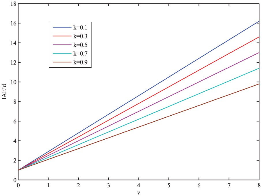
Relationship of $\mathrm{IA}{\mathrm{E}\prime }_{\mathrm{di}}-{\nu }_i$ based on different ${\kappa }_i$ values.

By substituting equation (52) into equation (51)

$$\mathrm{IA}{\mathrm{E}\prime }_{\mathrm{di}}=\underset{0}{\overset{\infty }{\int }}\left|{\zeta }^{-1}\left[\frac{1}{s}(1-\frac{{\rho }_{i}s+1}{{({\lambda }_{2i}s+1)}^2}{e}^{-{\theta }_{i}s})\right]\right|\mathrm{dt}$$

(53)

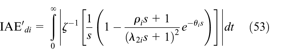
Equation (54) is obtained by calculating equation (53)

$$\mathrm{IA}{\mathrm{E}\prime }_{\mathrm{di}}=\{\begin{array}{c}{t}_i\hfill \\ \multicolumn{1}{c}{2{\lambda }_{2i}+{\theta }_i-{\rho }_i}\end{array}\begin{array}{c}{t}_i\le {\theta }_i\hfill \\ \multicolumn{1}{c}{t_i>{\theta }_i}\end{array}$$

(54)

When ${\lambda }_{2i}=-{\theta }_i/2$ and ${\rho }_i=0$ , the error between the disturbance and the output is maximum. When ${\rho }_i={\kappa }_i{\lambda }_{2i}$ , the relationship of $\mathrm{IA}{\mathrm{E}\prime }_{\mathrm{di}}-{\lambda }_{2i}$ can be obtained by

$$\frac{\mathrm{IA}{\mathrm{E}\prime }_{\mathrm{di}}}{{\theta }_i}=\{\begin{array}{c}{t}_i\hfill \\ \multicolumn{1}{c}{(2-{\kappa }_i){\nu }_i+1}\end{array}\begin{array}{c}{t}_i\le {\theta }_i\hfill \\ \multicolumn{1}{c}{t_i>{\theta }_i}\end{array}$$

(55)

where ${\lambda }_{2i}/{\theta }_i={\nu }_i$ .

According to equation (55), it is known that if $0<{\kappa }_i<2$ , then $min(\mathrm{IA}{\mathrm{E}\prime }_{\mathrm{ri}})=1$ ; if ${\kappa }_i>2$ , then $min(\mathrm{IA}{\mathrm{E}\prime }_{\mathrm{ri}})=0$ and ${\nu }_i=1/{\kappa }_i-2$ .

Robustness analysis

A TITO multivariable control system is nominally stable if and only if ²⁹

$$\rho =\left[\begin{array}{cc}0\hfill & \frac{G_{12}{C}_{11}}{1+G_{11}{C}_{11}}\hfill \\ \multicolumn{1}{c}{\frac{G_{21}{C}_{22}}{1+G_{22}{C}_{22}}}& 0\hfill \end{array}\right]<1\forall \omega$$

(56)

A practical way ²⁹ to identify the closed-loop system robustness stability in the presence of process uncertainties is to lump multiple sources of uncertainty into a multiplicative form

$$\rho (K_{\mathrm{ii}}(I+G^{-1})G{\Delta }_I)<1\forall \omega$$

(57)

$$\rho (G{K}_{\mathrm{ii}}(I+G^{-1}){\Delta }_O)<1\forall \omega$$

(58)

where Δ _I and Δ _O are stable process multiplicative input and output uncertainties, respectively. Hence, for a specified bound of Δ _I or Δ _O , control system robustness stability is evaluated by observing the magnitude plots of the left sides of equations (57) and (58) with $\omega \in [0,+\propto ]$ , which should fall below unity.

Remark 3

From the aspect of computation amount, the proposed method is increased complexity as compared to standard decoupling structure available in the literature. However, the performance of the control system is improved. Thus, the proposed method shows a trade-off between the dynamic performance and system robustness.

Simulation example

We consider two simulation examples to show the simplicity and effectiveness of the proposed method. One is Wood and Berry (WB) column (methanol–water distillation column) ³⁰ and other one is Alatiqi subsystem distillation column. ³¹

Example 1

Taking WB column as an example, the matrix function expression of the plant model is shown in the following equation

$$G_p(s)=\left[\begin{array}{cc}\frac{12.8e^{-s}}{16.7s+1}\hfill & \frac{-18.9e^{-3s}}{21s+1}\hfill \\ \multicolumn{1}{c}{\frac{6.6e^{-7s}}{10.9s+1}}& \frac{-19.4e^{-3s}}{14.4s+1}\hfill \end{array}\right]$$

According to section “Diagonal decoupling control,” the decoupler of WB column can be obtained by

$$D(s)=\left[\begin{array}{cc}1\hfill & \frac{1.476(16.7s+1)e^{-2s}}{21.3s+1}\hfill \\ \multicolumn{1}{c}{\frac{0.33(14.2s+1)e^{-4s}}{10.89s+1}}& 1\hfill \end{array}\right]$$

Then, according to equation (5), the diagonal matrix $\overline{G}(s)$ of WB column is given by

$$\begin{array}{c}{\overline{g}}_{11}(s)=\frac{12.8e^{-s}}{16.7s+1}-\frac{6.237(14.36s+1)}{228.69s^2+31.89s+1}{e}^{-7s}\hfill \\ {\overline{g}}_{22}(s)=\frac{-19.4e^{-3s}}{14.4s+1}+\frac{9.745(16.7s+1)}{228.69s^2+31.89s+1}{e}^{-9s}\hfill \end{array}$$

Then, according to section “Model reduced-order method,” the reduced-order model of $\overline{G}(s)$ can be obtained by

$$\begin{array}{c}{\overline{g}}_{11}^r(s)=\frac{6.563}{10.529s+1}{e}^{-0.309s}\hfill \\ {\overline{g}}_{22}^r(s)=\frac{-9.656}{6.273s+1}{e}^{-4.266s}\hfill \end{array}$$

The Bode plots of the first loop and the second loop are shown in Figure 7. Figure 7(a) shows the frequency characteristics comparison between the original model and the reduced-order model in the first loop. Figure 7(b) shows the frequency characteristics between the original model and the reduced-order model in the second loop.

Figure 7.

Bode comparison diagram between original model and reduced-order model for WB system: (a) is the first loop of the WB system and (b) is the second loop of WB system.

Applying the HO-PI, ³² BLT, ³¹ and SAT ³³ controllers to WB system output responses to a unit step function in the first or second input is shown in Figures 8–11. The obtained results are compared with those of the proposed method. Figures 8–11 show the track performance of the control system for WB control system. Figure 8 shows the set-point response and control law of the first loop for WB control system. Figure 9 shows the set-point response and control law of the second loop for WB system. In Figures 8 and 9, the obtained results show that proposed method possesses the favorable track performance.

Figure 8.

Set-point response of the first loop for WB control system.

Figure 9.

Set-point response of the second loop for WB control system.

Figure 10.

Disturbance response of the first loop for WB control system.

Figure 11.

Disturbance response of the second loop for WB control system.

Figure 10 shows the disturbance response and control law of the first loop for WB control system. Figure 8 shows the disturbance response and control law of the second loop for WB control system. In Figures 10 and 11, the obtained results show that proposed method possesses the favorable ability of the disturbance rejection. The performance index of the set-point response for WB system is shown in Table 1.

Table 1.

Performance indexes for WB column.

Method	Loop	Kmi	TIi	TDi	λ 1i	λ 2i	Msi	IAE I	IAE d
HO-PI	1	0.57	0.027	–	–	–	–	15.44	19.84
	2	−0.11	−0.0085	–	–	–	–	8.51	10.35
BLT	1	0.375	0.045	–	–	–	–	25.83	38.94
	2	−0.075	−0.003	–	–	–	–	16.31	28.63
SAT	1	0.87	0.267	–	–	–	–	13.79	18.32
	2	−0.09	−0.0086	–	–	–	–	6.68	9.07
Proposed	1	0.41	0.074	0.001	1.75	0.72	1.31	11.34	15.91
	2	−0.12	−0.024	−0.023	2.84	4.91	1.53	4.69	7.48

IAE: integral absolute error.

To further investigate and evaluate the control performance at frequency, we impose the frequency responses on the control system. The impulse response diagram is shown in Figure 12.

Figure 12.

Impulse response diagram of WB control system: (a) is the Impulse response for the first loop of the WB system and (b) is the Impulse response for the second loop of WB system.

The impulse response of control system provides information about the output of WB control system at different frequencies. From impulse response, it can be seen that the magnitude of the proposed method is smaller than that of other three methods for both loops. For the stability being evaluated in the frequency domain, the Nichols charts of each control system are drawn in Figure 13. In Figure 13, the gain margin of the proposed method is 9.3 dB and the phase margin of the proposed method is 35° for the first loop; and then, for the second loop, the gain margin of the proposed method is 6.5 dB and the phase margin of the proposed method is 60°. The results show that the proposed method possesses the favorable stability and robustness.

Figure 13.

Nichols chart of WB control system: (a) is the Nichols chart for the first loop of the WB system and (b) is the Nichols chart for the second loop of WB system.

Example 2

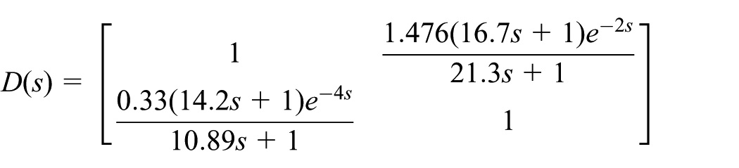
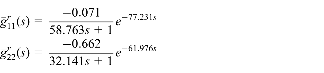
A modified Alatiqi subsystem distillation column is shown in the following equation

$$G(s)=\left[\begin{array}{cc}\frac{-0.51e^{-7.5s}}{{(32s+1)}^2(2s+1)}\hfill & \frac{1.68e^{-2s}}{{(28s+1)}^2(2s+1)}\hfill \\ \multicolumn{1}{c}{\frac{-1.25e^{-2.8s}}{(43.6s+1)(9s+1)}}& \frac{4.78e^{-1.15s}}{(48s+1)(5s+1)}\hfill \end{array}\right]$$

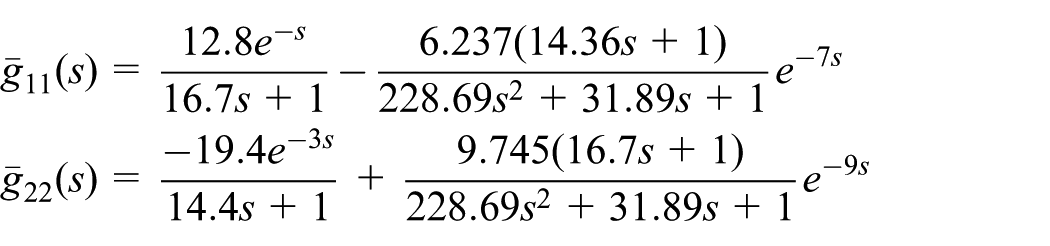
According to sections “Diagonal decoupling control” and “Model reduced-order method,” the decoupler matrix of Alatiqi subsystem can be given by

$$\begin{array}{c}D(s)=\left[\begin{array}{cc}1\hfill & \frac{3.294{(32s+1)}^2}{28s+1}\hfill \\ \multicolumn{1}{c}{\frac{0.262(48s+1)(5s+1)e^{-1.65s}}{(43.6s+1)(9s+1)}}& e^{-5.5s}\hfill \end{array}\right]\hfill \\ {\overline{g}}_{11}(s)=\frac{-0.51e^{-7.5s}}{(32s+1)(2s+1)}+\frac{0.439(48s+1)(5s+1)e^{-3.65s}}{{(28s+1)}^2(43.6s+1)(9s+1)(2s+1)}\hfill \\ {\overline{g}}_{22}(s)=\frac{4.78e^{-6.65s}}{(48s+1)(5s+1)}-\frac{4.118(32s+1)e^{-2.8s}}{{(28s+1)}^2(43.6s+1)(9s+1)}\hfill \end{array}$$

Then, the reduced-order model of $\overline{G}(s)$ can be obtained by

$$\begin{array}{c}{\overline{g}}_{11}^r(s)=\frac{-0.071}{58.763s+1}{e}^{-77.231s}\hfill \\ {\overline{g}}_{22}^r(s)=\frac{-0.662}{32.141s+1}{e}^{-61.976s}\hfill \end{array}$$

The Bode plots of the first loop and the second loop are shown in Figure 14. Figure 14(a) shows the frequency characteristics between the original model and the reduced-order model in the first loop. Figure 14(b) shows the frequency characteristics between the original model and the reduced-order model in the second loop.

Figure 14.

Bode comparison diagram between original model and reduced-order model for Alatiqi subsystem: (a) is the first loop of the Alatiqi subsystem and (b) is the second loop of Alatiqi subsystem.

Applying the MV, ³⁴ NDT, ²² and Wang ³⁵ controllers to the modified Alatiqi subsystem output responses to a unit step function in the first or second input is shown in Figures 12–15. The results are compared with those of the proposed method. Figures 15–18 show the track performance of the control system for the modified Alatiqi subsystem.

Figure 15.

Set-point response of the first loop for Alatiqi subsystem.

Figure 16.

Set-point response of the second loop for Alatiqi subsystem.

Figure 17.

Disturbance response of the first loop for Alatiqi subsystem.

Figure 18.

Disturbance response of the second loop for Alatiqi subsystem.

Figure 15 shows the set-point response and control law of the first loop for the modified Alatiqi subsystem. Figure 16 shows the set-point response and control law of the second loop for the modified Alatiqi subsystem. In Figures 15 and 16, the obtained results show that proposed method shows the trade-off between the dynamic performance and robustness. Figure 17 shows the disturbance response and control law of the first loop for the modified Alatiqi subsystem. Figure 18 shows the disturbance response and control law of the second loop for the modified Alatiqi subsystem.

In Figures 17 and 18, the obtained results show that proposed method possesses the favorable ability of the disturbance rejection. The performance index of the set-point response for the modified Alatiqi control system is shown in Table 2.

Table 2.

Performance indexes for Alatiqi subsystem.

Method	Loop	Kmi	TIi	TDi	λ 1i	λ 2i	Msi	IAE I	IAE d
MV	1	−2.12	−0.03	–	–	–	–	22.36	31.64
		−0.126	0.013	0.467	–	–	–
	2	−0.218	−0.009	0.624	–	–	–	25.04	36.19
		0.049	0.004	–	–	–	–
NDT	1	−6.393	−0.092	–	–	–	–	18.03	23.42
	2	0.499	0.012	–	–	–	–	21.72	30.37
Wang	1	−2.176	−0.059	0.807	–	–	–	15.94	21.79
	2	0.154	0.005	−0.117	–	–	–	19.08	24.04
Proposed	1	−2.14	−0.046	0.913	5.965	134.298	1.39	17.16	22.95
	2	0.504	0.0089	−0.091	8.378	65.850	1.63	20.67	28.47

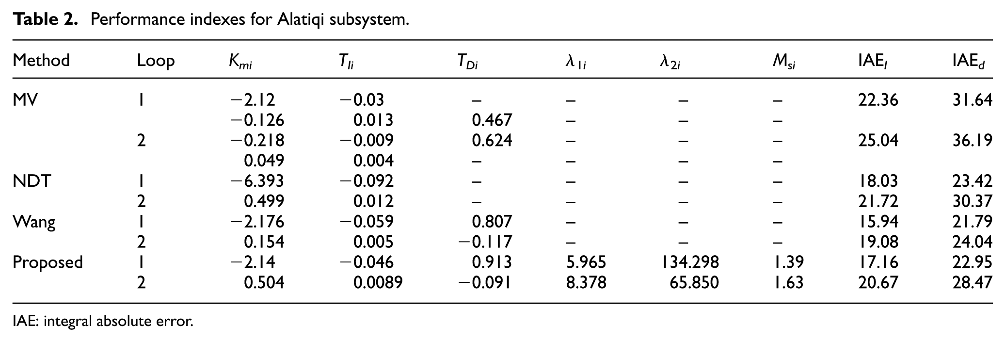
IAE: integral absolute error.

To further investigate and evaluate the control performance at frequency, we impose the frequency responses on the control system. The impulse response diagram is shown in Figure 19. For the stability being evaluated in the frequency domain, the Bode diagrams of each control system are shown in Figure 20.

Figure 19.

Impulse response diagram of Alatiqi subsystem: (a) is the impulse response for the first loop of the Alatiqi subsystem and (b) is the impulse response for the second loop of Alatiqi subsystem.

Figure 20.

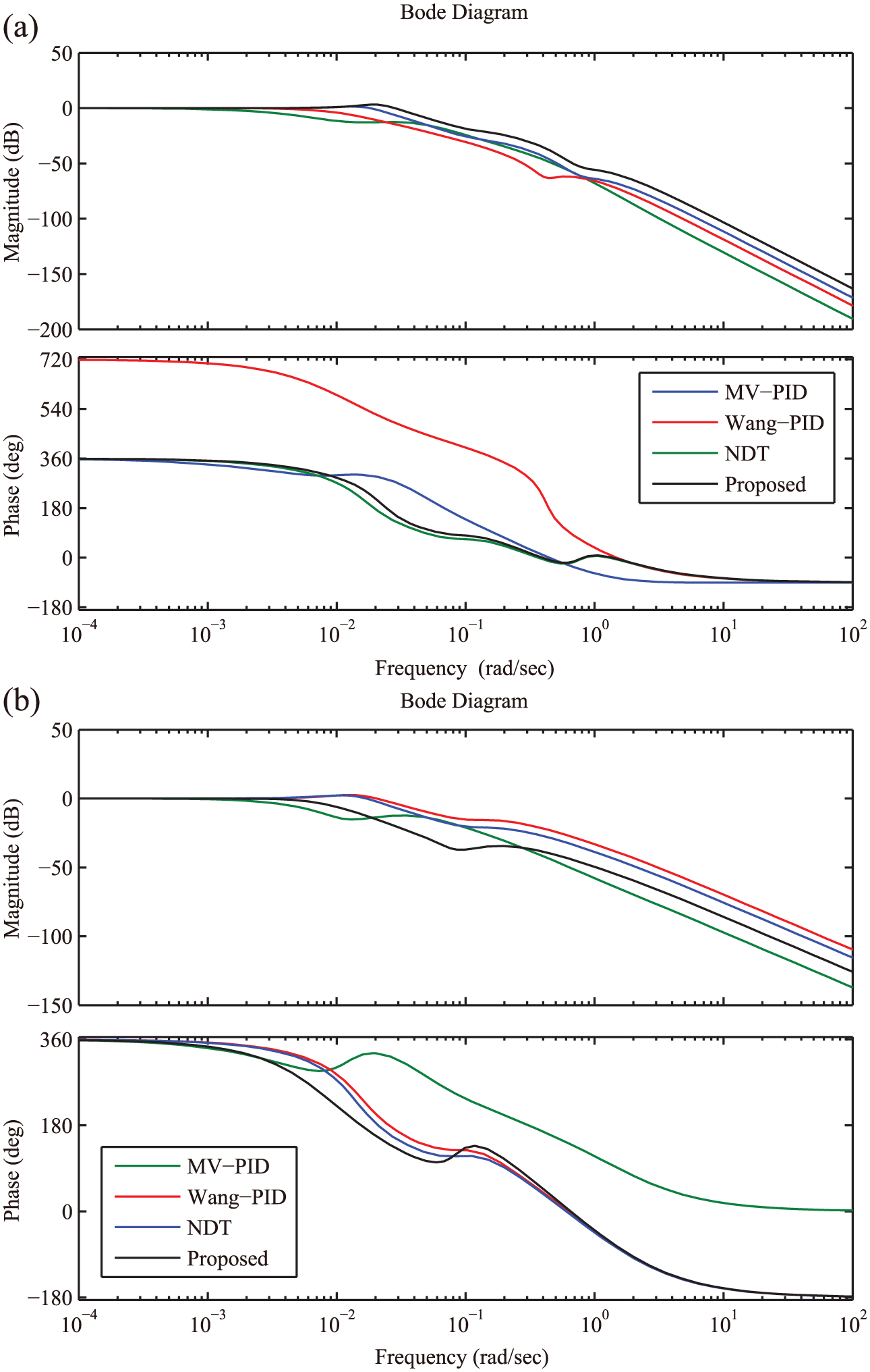
Bode diagram of Alatiqi subsystem: (a) is the Bode diagram for the first loop of the Alatiqi subsystem and (b) is the Bode diagram for the second loop of Alatiqi subsystem.

According to the simulation results of Examples 1 and 2, it is observed that the proposed method can improve the anti-interference ability and realize the effectiveness of the ADR. However, the improvement of the anti-interference ability is at the cost of losing the partial dynamic performance. Hence, the proposed method shows a trade-off between the dynamic performance and system robustness.

Conclusion

In this article, a compound control structure of ADRIMC is proposed and applied to TITO system with time delay process for improving the system robustness. The decoupler matrix method is applied to decoupled TITO system, and then, Maclaurin series reduced-order method is used to find an equivalent FOPDT for each loop. The controller parameters are tuned by IMC-PID technique. Using this design method, the system robustness is improved on the structure uncertainty aspect of the control system. Further research extending the presented methodology to the design of multivariable controllers for $n\times n$ dimension system and non-square systems with large model errors is currently ongoing.