Sage Journals: Discover world-class research

Abstract

For pump–turbines, most of the instabilities couple with high-level pressure fluctuations, which are harmful to pump–turbines, even the whole units. In order to understand the causes of pressure fluctuations and reduce their amplitudes, proper numerical methods should be chosen to obtain the accurate results. The method of large eddy simulation with wall-adapting local eddy-viscosity model was chosen to predict the pressure fluctuations in pump mode of a pump–turbine compared with the method of unsteady Reynolds-averaged Navier–Stokes with two-equation turbulence model shear stress transport k–ω. Partial load operating point (0.91Q_BEP) under 15-mm guide vane opening was selected to make a comparison of performance and frequency characteristics between large eddy simulation and unsteady Reynolds-averaged Navier–Stokes based on the experimental validation. Good agreement indicates that the method of large eddy simulation could be applied in the simulation of pump–turbines. Then, a detailed comparison of variation for peak-to-peak value in the whole passage was presented. Both the methods show that the highest level pressure fluctuations occur in the vaneless space. In addition, the propagation of amplitudes of blade pass frequency, 2 times of blade pass frequency, and 3 times of blade pass frequency in the circumferential and flow directions was investigated. Although the difference exists between large eddy simulation and unsteady Reynolds-averaged Navier–Stokes, the trend of variation in different parts is almost the same. Based on the analysis, using the same mesh (8 million), large eddy simulation underestimates pressure characteristics and shows a better result compared with the experiments, while unsteady Reynolds-averaged Navier–Stokes overestimates them.

Keywords

Pump–turbine pump mode pressure fluctuation large eddy simulation unsteady Reynolds-averaged Navier–Stokes

Introduction

With the rapid development of pumped storage power plants, pump–turbines as the key part trend to higher head, larger capacity, and higher specific speed. However, several problems arise obviously in the operations of pump–turbines, such as hump instability in pump mode, S-shaped instability in turbine mode, and corresponding high-level pressure fluctuations in both the modes. In order to ensure the safe and effective operation, it is significantly important to study the causes of these strong pressure fluctuations. Nevertheless, the first thing is to find a proper method to predict the accurate pressure characteristics.

With the development of computational fluid dynamics (CFD), it has become the primary method of studying pressure fluctuations in pump–turbines. Lots of studies have been carried out to investigate the pressure characteristics, and they indicate the highest level pressure fluctuations occur in the vaneless space of pump–turbines, which generally come from the rotor stator interaction (RSI).¹ Additionally, some other pressure fluctuations induced by rotating stall,² vortex rope,³ and misaligned guide vanes (MGVs)⁴ were also presented through experimental and numerical methods.

However, almost all numerical studies are based on the method of unsteady Reynolds-averaged Navier–Stokes (URANS), which has often been reported to overpredict pressure characteristics compared with the experimental data. Sun et al.⁵ presented the distribution of pressure fluctuations in a pump–turbine in pump mode using URANS with two-equation turbulence model shear stress transport (SST) k–ω. In his research, the calculated amplitudes of dominant frequencies are much higher than the experiments. Guo et al.⁶ obtained the detailed propagation of pressure fluctuations of a pump–turbine in pump mode through the same turbulence model. Then, still the same numerical method was used to study the pressure characteristics in hump instability region by Li et al.⁷ Meanwhile, pressure fluctuations of a pump–turbine in turbine mode with MGV were investigated using $\bar{v^{2}} - f$ turbulence model⁸ and SST turbulence model.⁴

Recently, large eddy simulation (LES), a relatively new type of numerical simulation, is developed rapidly. In LES, Navier–Stokes (N-S) equations are filtered depending on the filter spatially, such as the classical Deardorff⁹ filter. Large-sized eddies are solved directly by controlling equations, and small-sized eddies are simulated through sub-grid scale (SGS) models. As a transitional method between Reynolds-averaged Navier–Stokes (RANS) and direct numerical simulation (DNS), LES has been studied in analyzing simple fundamental flows, such as turbulent mixing layers⁹ and channel flows.^10,11 However, it requests longer computational time and more accurate mesh generation. Up to now, little attention was paid to the applications in the industry, especially in the hydraulic machinery.

An LES of a turbulent flow past an airfoil near stall at a chord was performed and compared with wind–tunnel experiments. Its explicit selective mixed scale model (SMSM) was approved to be the first satisfying LES of relatively complex flow.¹² Byskov et al.¹³ investigated a shrouded six-bladed centrifugal pump impeller using LES and reproduced the stall phenomenon observed at quarter load which can be absurd by RANS models.

In the pump, unsteady numerical calculation of an entire multistage pump was performed using LES focusing on the turbulence field evolution inside the impeller.^14,15 Predictions of LES suggest that Boussinesq’s hypothesis does not seem to be valid, especially near the exit of the impeller where the blade unloading takes place. Abramian and Howard¹⁶ applied LES in a turbulent flow through a complete Francis turbine including spiral casing, runner, and draft tube and assessed the validity with measurements on the velocity distribution. Song et al.¹⁷ concluded that LES could predict small phenomenon such as vortex dynamics which guides the design of the Francis turbine. Pacot et al.¹⁸ accurately reproduced phenomenon of rotating stall for a reduced Reynolds number using the LES approach with acceptable computing resources. Jang et al.¹⁹ proved the validity of the LES with experiments using laser Doppler velocimetry (LDV) measurements for analyzing three-dimensional structures of the vertical flow field in a propeller fan with a shroud covering only the rear region of its rotor tip. For the sub-grid model test, Bensow and Liefvendahl²⁰ performed explicit and implicit modeling. It confirmed that implicit modeling gives a better prediction of the global performance of the propeller. As a conclusion, LES could be applied in simulating in pump–turbines. Moreover, some efforts have been carried out in pump–turbines.

For pump–turbines, most of the instabilities, such as hump and S-shaped instabilities, couple with high-level pressure fluctuations, which are harmful to pump–turbines. To obtain more accurate pressure fluctuations, the method of LES was chosen in this research to assess the feasibility in simulating pump characteristics of a pump–turbine. Based on the experimental validation, frequency characteristics of the whole water passage were analyzed using the method of LES and URANS.

Numerical simulation

Numerical model

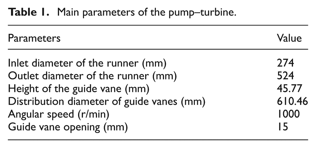
The pump–turbine model consists of a spiral casing, a runner with 9 blades, 20 adjustable guide vanes, 20 stay vanes including a special stay vane, and a draft tube. The specific speed n_q = 30.7 is calculated according to equation (1). The computational domain is shown in Figure 1. Table 1 lists the main parameters of the pump–turbine

n_{q} = \frac{n \sqrt{Q}}{H^{3 / 4}}

(1)

where Q is the discharge of optimum efficiency point in pump mode (m³/s), H is the head (m), and n is rotational speed (r/min).

Figure 1.

Computational domain of the pump–turbine.

Table 1.

Main parameters of the pump–turbine.

Parameters	Value
Inlet diameter of the runner (mm)	274
Outlet diameter of the runner (mm)	524
Height of the guide vane (mm)	45.77
Distribution diameter of guide vanes (mm)	610.46
Angular speed (r/min)	1000
Guide vane opening (mm)	15

Mesh information

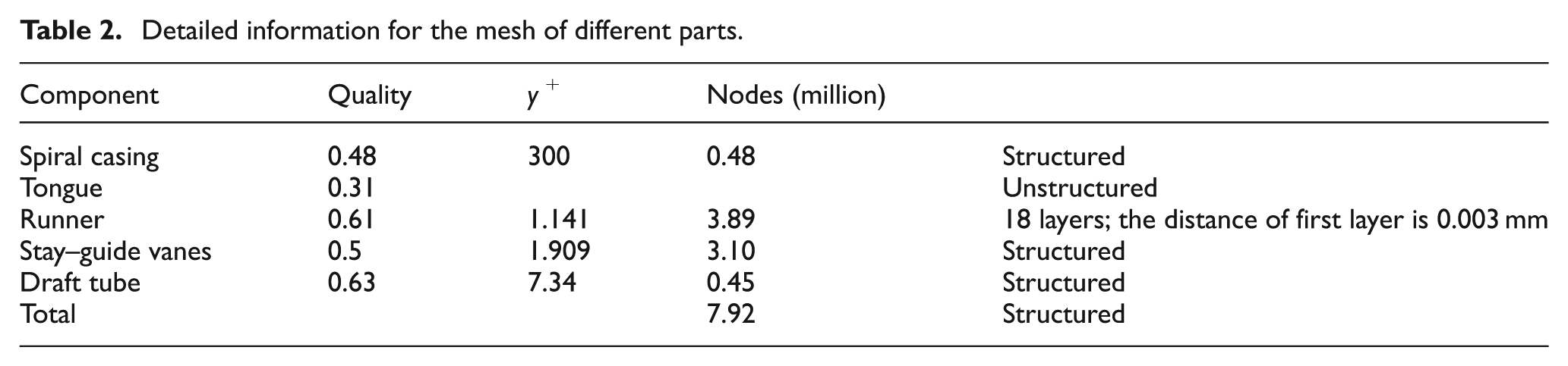
The meshes for all the parts were generated by ANSYS 14.0 module ICEM. Because of the sharp shape of the spiral casing tongue, an adapted mesh was created using unstructured tetrahedral cells. The distance of the first layer off the solid wall is 0.003 mm for runner blades and stay–guide vanes. y⁺ in average in the runner and stay–guide vanes is less than 2. The total number of nodes of the mesh is 7.92 million. Table 2 reports the detailed information for all the parts.

Table 2.

Detailed information for the mesh of different parts.

Component	Quality	y⁺	Nodes (million)
Spiral casing	0.48	300	0.48	Structured
Tongue	0.31		0.48	Unstructured
Runner	0.61	1.141	3.89	18 layers; the distance of first layer is 0.003 mm
Stay–guide vanes	0.5	1.909	3.10	Structured
Draft tube	0.63	7.34	0.45	Structured
Total			7.92	Structured

Boundary conditions

In the LES simulation, spectral synthesizer was chosen to generate the fluctuating velocity at the draft inlet. The rest of the boundary conditions are the same with the ones used in the URANS simulation. Mass flow inlet was used at the draft tube (pump mode) according to the experimental data. The turbulence option was specified as intensity (2%) and hydraulic diameter (280.5 mm) at the inlet. Static pressure (0 Pa) at spiral casing outlet was set. No-slip wall conditions were imposed for all the remaining solid walls.

Numerical setup

The chosen SGS model is very important to the numerical results. Wall-adapting local eddy-viscosity (WALE) model, which is based on the square of the velocity gradient tensor, was proposed by Nicoud and Ducros²¹ and has a proper near wall behavior. The WALE model is invariant to any coordinate translation or rotation, and only local information is needed so that it is well suited for LES in complex geometry.²² Due to the complex geometry of pump–turbines, this model is suitable for this study.

In the LES simulation, the spatial discretization scheme is second order for pressure and least squares cell based for gradient. Bounded central differencing is chosen for momentum because it could produce a low numerical diffusion.²³ Under-relaxation factors for pressure, density, bodyforce, and momentum are 0.3, 1, 1, and 0.7, respectively. In the URANS simulation, under-relaxation factors for pressure, density, bodyforce, and momentum are the same with the ones in LES. In addition, for turbulent kinetic energy, it is 0.8. Second upwind for momentum, turbulent kinetic energy, and specific dissipation rate terms was set for spatial discretization schemes. For pressure and gradient, schemes are also the same with the ones in LES. In both the methods, SIMPLEC algorithm was used for pressure–velocity coupling, and the residual criterion was set as 10⁻⁶ with 100 internal iterations. Time step was set as 0.0002 s corresponding to 1.2° of rotation for the runner per step.

Mesh validation

Five sets of girds with different number of nodes were created using ANSYS 14.0 module ICEM to test the grid independence. The variation of performance characteristic parameters (head and efficiency) versus the number of nodes is presented in Figure 2. For the head of the pump–turbine, in the SST k–ω simulation, as the number of the nodes is increased, the head increases; in the LES simulation, with the increase in the number, the head decreases. When the number reaches 8 × 10⁶, the heads are very close to experimental value (42.82 m), and the errors are, respectively, −0.48% and 0.19% for SST k–ω and LES simulations compared with experiments. With respect to the efficiency of the pump–turbine, for both the methods, the efficiencies increase with the increase in the number. For the 8 million of nodes, the efficiencies are also close to the experiments, and the errors are <1.5% (0.12% for SST k–ω, 1.13% for LES). Based on the above validation, the fifth set of grid was used in simulations.

Figure 2.

Variation of (a) head and (b) efficiency with the number of the nodes, experimental head is 42.82 m and efficiency is 88.95% for the validated point under 15-mm guide vane opening.

Additionally, in LES simulation, the accuracy of the mesh shows much more important due to the requirements of LES. Two sets of grids were validated using other methods in this research. The number of the coarse mesh is 4.5 million, and the fine one is 8 million as shown in Figure 3. The contours of vorticity for different meshes are shown in Figure 4. In Figure 4(a), small flow separation regions could be observed only around the blades and vanes. Unlike the second mesh (Figure 4(b)), small vortices in the passages of the runner and vanes could be captured in the simulations.

Figure 3.

Meshes for different number of the nodes: (a) 4.5 million and (b) 8 million.

Figure 4.

Vorticity distribution for different number of the nodes: (a) 4.5 million and (b) 8 million.

The SGS viscosity to water molecular viscosity is shown in Figure 5. The closer to 1 the value of $ν_{sgs} / ν$ , the more the accuracy for the simulation. From Figure 5, the values for most regions are close to 1 for the two meshes, although some small high-value areas still exist. Considering the capacity of the computer and the vortex scale in pump–turbines, the second mesh was chosen in the following simulations.

Figure 5.

$ν_{sgs} / ν$ distribution for different number of the nodes: (a) 4.5 million and (b) 8 million.

Experimental validation

Validation of performance characteristics

Partial discharge operating point 0.91Q_BEP under 15-mm guide vane opening was simulated in this research. For the pump–turbine, 27-mm guide vane opening is optimum, where the maximum efficiency is 91.57%. Hence, 15 mm is relatively small guide vane opening. Performance curves under 15-mm guide vane opening are shown in Figure 6. Point 0.91Q_BEP is a turn point (wave peak) in the head–discharge curve. In order to validate the accuracy of the numerical simulations, the experimental data obtained from Harbin Institute of Large Electrical Machinery (HILEM) were compared with the numerical results in Figure 6. The detailed information of comparison is shown in Table 3. Subscripts “Sim” and “Exp” stand for the results from simulations and experiments, respectively. Subscript “Error” denotes the error between the numerical and experimental data, which is defined as follows

Φ_{Error} = \frac{(Φ_{Sim} - Φ_{Exp})}{Φ_{Exp}} \times 100 %

(2)

Figure 6.

Performance curves of the pump–turbine in pump mode.

Table 3.

Comparison between simulations and experiments.

GVO		LES	URANS	LES	URANS
GVO	H_Exp (m)	H_Sim (m)		H _Error
15 mm	44.20	45.06	41.04	1.95	−7.15
	T_Exp (N m)	T_Sim (N m)		T _Error
	821.21	821.50	814.23	0.04	−0.85
	η _Exp	η _Sim		η _Error
	88.23	90.93	83.51	3.06	−5.35

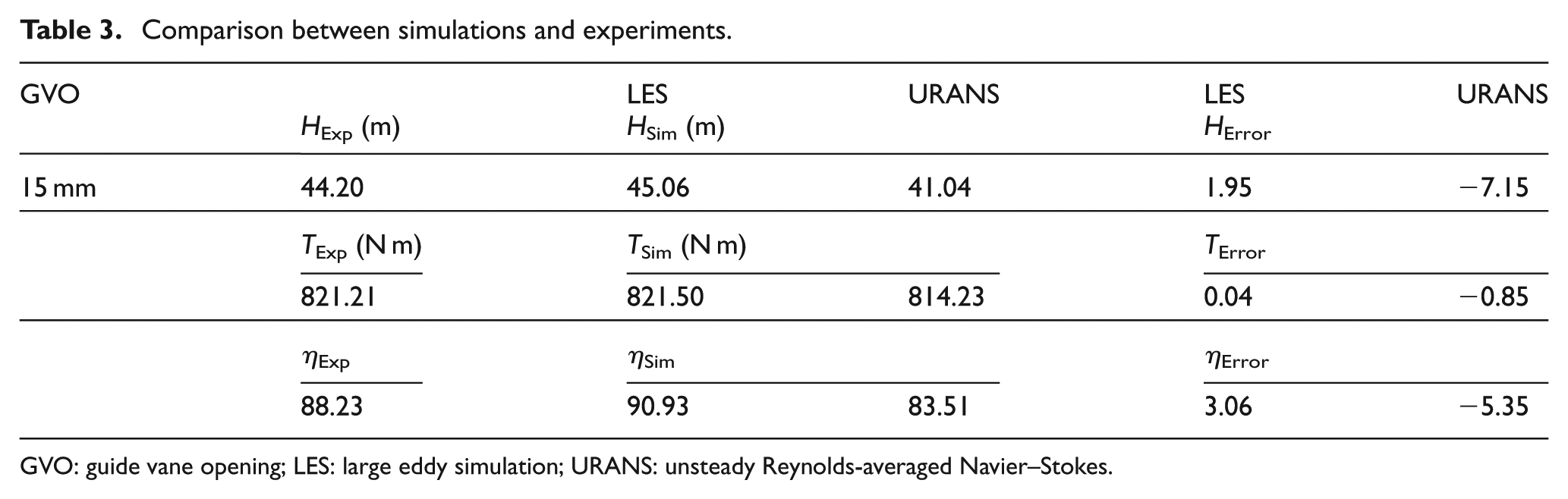
GVO: guide vane opening; LES: large eddy simulation; URANS: unsteady Reynolds-averaged Navier–Stokes.

Where, Φ represents H, T and η. As listed in Table 3, the head error predicted in LES simulation compared with experiments is 1.95%, while for URANS, it is −7.15%. The torque errors for both the methods are <1%. It is 0.04% for the LES and −0.85% for the URANS. With respect to efficiency, the errors are >3% (3.06% for LES, −5.35% for URANS) due to simplification of geometry of the pump–turbine in the simulations. In sum, all the numerical results from the LES show better than URANS, especially for the torque. Furthermore, LES overpredicts all the performance characteristics, while URANS underestimates them. Nevertheless, the accuracies between the numerical simulations and experiments for both the methods are in a reasonable range in predicting the performance characteristics.

Validation of pressure fluctuations

In order to validate the feasibility for prediction of pressure characteristics, eight sensors were set in the experiments as shown in Figure 7. A total of two points were set in the elbow of the draft tube, two points in the cone of the draft tube, two points in vaneless space between the runner outlet and guide vane inlet, one point in the channel of the stay vanes, and one point in the outlet of the spiral casing. Experiments of pressures fluctuations were carried out in HILEM. All the sensors were calibrated before the experiments. The sampling rate is 4000 Hz, and the number of the sampling is 40,000. ΔH indicates peak-to-peak value for the pressure fluctuation of pressure–time signal. Generally, ΔH/H is used to show the relative value of the pressure fluctuation. Point 0.91Q_BEP was chosen in this study to make a comparison between different numerical methods and experiments. Based on the results of RANS, the simulation of URANS was performed for 15 revolutions. The remaining eight revolutions were used to analyze the pressure characteristics. A comparison of ΔH/H between the simulations and experiments for eight monitoring points is shown in Figure 8. The highest level pressure fluctuation occurs between runner outlet and guide vane inlet (RG1, RG2), which mainly results from RSI.²⁴ In the draft tube, both the methods could better predict the value of ΔH/H (see Figure 8). In the vaneless space, LES shows a bit better performance, where the values are closer to experiments. However, both show a large error in spiral casing and stay vanes. Nevertheless, it can be concluded that the tendency of variation is almost the same for numerical results and experiments. The pressure fluctuation increases from draft tube to vaneless space and then decreases to the spiral casing.

Figure 7.

Monitoring points in the experiments.

Figure 8.

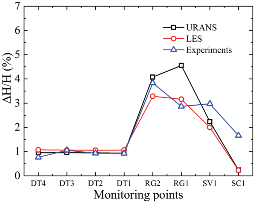
Comparison of peak-to-peak value between simulations and experiments.

The nondimensional coefficient of pressure fluctuation is defined according to equation (3), which stands for how much the pressure fluctuations relative to the kinetic energy at the runner outlet

C_{p} = \frac{p - \bar{p}}{\frac{1}{2} ρ u_{2}^{2}} \times 100 %

(3)

where p is the instantaneous pressure (Pa), $\bar{p}$ is the averaged pressure (Pa), ρ is the density (kg/m³), and u₂ is the circumferential velocity at the runner outlet (m/s).

Figure 9 depicts frequency spectrum for different monitoring points between numerical results and experiments. For all the monitoring points, the amplitudes of dominant frequencies predicted by URANS are larger than experiments, while the ones obtained from LES are lower. This may be the reason that LES overestimates the performance characteristics, while URANS underestimates them as shown in Table 3. Besides the point in the spiral casing, blade pass frequency (BPF) and its harmonic frequencies (2BPF and 3BPF) could be predicted very well.

Figure 9.

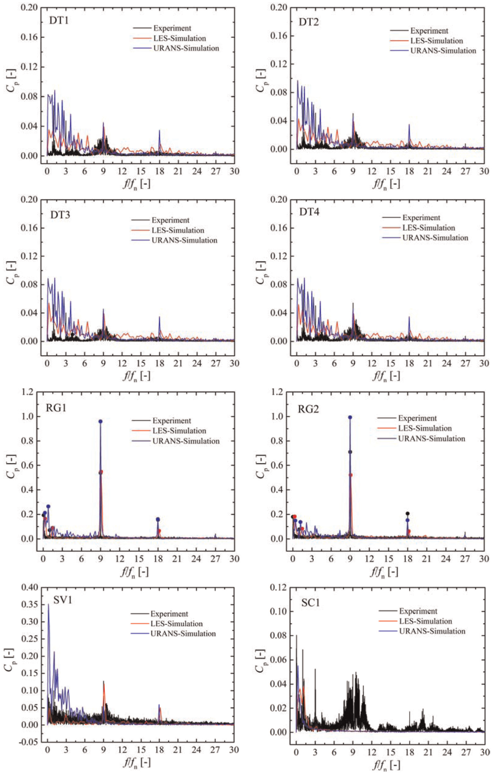
Comparison of frequency spectrum between simulations and experiments.

In the draft tube, both the methods of LES and URANS overestimate the dominant frequencies. In the experiments, two low frequencies (1.16f_n and 3f_n) could be observed, which are not well predicted by both the methods. In both the simulations, complex low frequencies are found, which may be related to boundary conditions (inlet turbulence intension).

In the vaneless space, all the dominant frequencies from both the simulations agree well with experiments, especially the first dominant frequency (BPF) and second dominant frequency (0.1f_n). Moreover, URANS overestimates most of the dominant frequencies, while LES underestimates them and shows closer to experiments. In this part, the mesh was refined, and the numerical results agree well with experimental data.

In the stay vanes, the extremely high amplitude 0.12f_n could be found in URANS, while this frequency is not so high in LES and experiments. It can be also seen that BPF and 2BPF predicted for both the methods agree with the experiments.

In the spiral casing, both the methods underestimate the value. Only two low frequencies could be predicted well. BPF and its harmonic frequencies could be not obtained in both the methods, while they feature obviously high amplitudes in the experiments. This may be due to poor mesh in this part.

In sum, both the methods could better predict dominant frequencies, especially in vaneless space. Due to the little number of the nodes in the draft tube and spiral casing, the numerical results are not very good compared with the experimental data. Nevertheless, BPF and its harmonic frequencies could be well predicated in the whole passage except spiral casing part.

Results and discussion

Monitoring points in the simulations

To obtain more detailed information between LES and URANS, more monitoring points were set in the whole passage. A total of 8 points were set in the spiral casing and named from SC1 to SC8, 34 points between runner outlet and guide vane named from VL1 to VL34 at the circumference, 10 groups of points in guide vane passages named from GV1 to GV50, and 19 points in stay vane passages named from SV1 to SV19. The detailed distribution for monitoring points is depicted in Figure 10. In the guide vane passages, for every group of points, the number decreases from guide vane inlet to outlet (pump mode).

Figure 10.

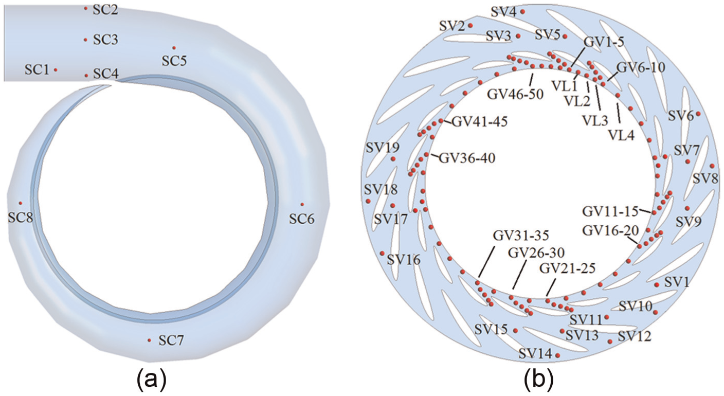
Monitoring points in the simulations: (a) in the spiral casing and (b) in stay and guide vanes.

Variation of peak-to-peak value

Variation of peak-to-peak pressure fluctuations in the whole passage is shown in Figure 11. From Figure 11(a), in the spiral casing, the tendency of variation is the same for LES and URANS, and the difference between the two methods is small. From the spiral casing outlet to the spiral tongue, ΔH/H shows an obvious increase, which indicates the sharp shape of the spiral tongue has an obvious impact on pressure fluctuations.

Figure 11.

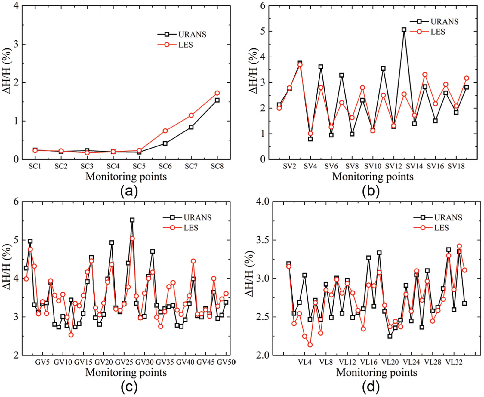
Variation of peak-to-peak value in the whole passage: (a) variation in spiral casing, (b) variation in stay vanes, (c) variation in guide vanes, and (d) variation in vaneless space.

From Figure 11(b), in the stay vane passages, ΔH/H decreases along the flow direction. The tendency for both the methods is almost the same; only the amplitudes for several points show a large difference. For URANS, the amplitudes of four points (SV5, SV7, SV11, and SV13) are obviously higher than the ones from LES.

From Figure 11(c), in the guide vane passages, for every group of monitoring points, ΔH/H increases from the first point to the second point along the flow direction, and then it decreases from the third point to the fourth point; finally, it increases again from the fourth point to fifth point.

From Figure 11(d), in the vaneless space between runner outlet and guide vane inlet, the variation of ΔH/H is periodic for both the methods. The values predicted by LES are much smaller than the ones through URANS. In addition, the values close to special stay vane are larger than the remaining ones for both the methods. This indicates that vortices occur in the channels around the special stay vane.

Although the difference exists between LES and URANS, the tendency of the variation in different parts is almost the same. It shows that both the methods could better predict the variation of pressure fluctuations.

Propagation of BPF, 2BPF, and 3BPF

Based on the above analysis, both the methods could better predict BPF and its harmonic frequencies, especially in the vaneless space. Additionally, the highest level pressure fluctuations occur in the vaneless space, which mainly come from RSI between guide vanes and runner blades. Hence, propagation of BPF, 2BPF, and 3BPF is compared between LES and URANS in the circumferential and flow directions. Figure 12 shows the distribution of BPF at the circumference. It can be noticed that most of the amplitudes from URANS are larger than the ones from LES. Two high-amplitude regions could be noted for both the methods. Although the amplitudes between the two methods are different, the variation of distribution is similar. In addition, the difference between the high-amplitude region and low-amplitude region is much more obvious from URANS than the one from LES.

Figure 12.

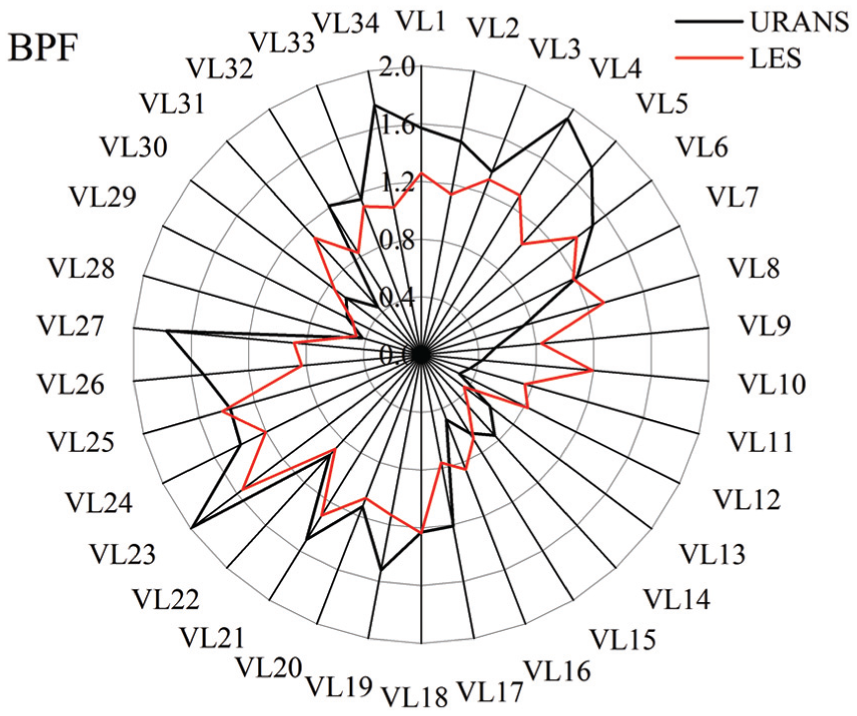
Distribution of BPF at the circumference.

Figure 13 presents the distribution of 2BPF in the vaneless space. The distribution is also almost the same for both the methods. Also, the amplitudes between the two methods are closer than the ones for BPF. For LES, four high-amplitude regions could be distinguished. The distribution of 3BPF at the circumference is depicted in Figure 14. Although the variation is still the similar for both the methods, the amplitudes obtained from LES change larger than the ones from URANS. The distribution for both the methods shows a little difference.

Figure 13.

Distribution of 2BPF at the circumference.

Figure 14.

Distribution of 3BPF at the circumference.

The distribution of amplitudes of BPF, 2BPF, and 3BPF along the flow direction is given in Figure 15. For both the methods, the amplitudes of BPF increase sharply from the draft tube to the vaneless space and show a decline along the guide vane passage and then have a quick drop in the stay vanes and the spiral casing. For LES, the tendency is almost the same with the one in URANS. Only from the outlet of stay vanes to the spiral casing outlet, the amplitude keeps no change. The variation of 2BPF is almost the same with BPF. The amplitudes in the guide vanes and stay vanes from URANS become larger than the ones from LES. For 3BPF, the amplitudes of all the points from LES are almost the same with the ones from URANS. Nevertheless, the tendency of BPF, 2BPF, and 3BPF along the flow direction is almost the same for both the methods, which is similar with the one predicted in another pump–turbine in pump mode by Sun et al.⁵

Figure 15.

Propagation of BPF, 2BPF, and 3BEP along the flow direction.

Conclusion

This study presents the difference in pressure fluctuation in pump mode of a pump–turbine between the methods of LES with WALE model and URANS with two-equation turbulence model SST k–ω. Based on the experimental validation, performance characteristics and BPF and its harmonic frequencies could be predicted by both the methods. Moreover, LES has some advantages in predicting performance characteristics, and the amplitudes of BPF and its harmonic frequencies are much closer to the experiment data.

A comparison of variation of peak-to-peak value for pressure fluctuation in the whole passage shows that the tendency of variation in different parts for both the methods is almost the same. The propagation of amplitudes of BPF, 2BPF, and 3BPF in the circumferential and flow directions is also similar. It can be concluded that the method of LES could be applied in simulating pump–turbines.

However, it is also found that URANS underestimates performance characteristics and overestimates pressure fluctuations, while LES is opposite for these characteristics. This might result from the mesh. Both the methods use the same mesh, but the requirements of LES and URANS simulations are different. Using 8 millions of nodes, URANS could better predict vortices in the whole passage. Hence, performance characteristic parameters obtained from URANS are lower than the experiments, and frequency amplitudes are higher than the experiments.

A further study should be continued in the next step. The number of nodes should be added in the whole passage for the method of LES. Some schemes of LES should be improved to obtain better results compared with the experiments. Moreover, some monitoring points in the runner should be added to make a comparison between LES and URANS.

Footnotes

Academic Editor: Sergio Nardini

Declaration of conflicting interests

The author(s) declared no potential conflicts of interest with respect to the research, authorship, and/or publication of this article.

Funding

The author(s) disclosed receipt of the following financial support for the research, authorship, and/or publication of this article: This work was supported by Foundation for Innovative Research Groups of the National Natural Science Foundation of China (grant no. 51121004).

References

Zuo

Liu

Sun

. Pressure fluctuations in the vaneless space of high-head pump-turbines—a review. Renew Sustain Energ Rev 2015; 41: 965–974.

Xia

Cheng

Zhang

. Numerical analysis of rotating stall instabilities of a pump-turbine in pump mode. IOP C Ser Earth Env 2014; 22: 032020.

Kirschner

Ruprecht

Gode

. Experimental investigation of pressure fluctuations caused by a vortex rope in a draft tube. IOP C Ser Earth Env 2012; 15: 062059.

Xiao

Wang

Zhang

. Numerical predictions of pressure pulses in a Francis pump turbine with misaligned guide vanes. J Hydrodyn B 2014; 26: 250–256.

Sun

Zuo

Liu

. Distribution of pressure fluctuations in a prototype pump turbine at pump mode. Adv Mech Eng. Epub ahead of print 11 February 2014. DOI: 10.1155/2014/923937.

Guo

Liu

Wang

. Pressure fluctuation propagation of a pump turbine at pump mode under low head condition. Sci China Technol Sci 2014; 57: 811–818.

Wang

Xiang

. Frequencies spectrum analysis for hump characteristic in a pump turbine. In: 6th international symposium on fluid machinery and fluid engineering, Wuhan, China, 22–22 October 2014. New York: IEEE.

Liu

Sun

. Numerical simulation of pressure fluctuation of a pump-turbine with MGV at no-load condition. IOP C Ser Earth Env 2012; 15: 062036.

Deardorff

JW.

A numerical study of three-dimensional turbulent channel flow at large Reynolds numbers. J Fluid Mech 1970; 41: 453–480.

10.

Hamba

A hybrid RANS/LES simulation of turbulent channel flow. Theor Comp Fluid Dyn 2003; 16: 387–403.

11.

McCoy

Constantinescu

Weber

Coherent structures in a channel with Groyne fields: a numerical investigation using LES. In: Impacts of global climate change, Anchorage, AK, 15–19 May 2005. Reston, VA: ASCE.

12.

Kang

QJ.

Large eddy simulation of the turbulent flow around a circular cylinder at sub-critical Reynolds numbers. Acta Mech Sinica 1999; 15: 100–105.

13.

Byskov

Jacobsen

Pedersen

Flow in a centrifugal pump impeller at design and off-design conditions—part II: large eddy simulations. J Fluid Eng: T ASME 2003; 125: 73–83.

14.

Nagahara

Inoue

Sato

. Investigation of the flow field in a multistage pump by using LES. In: ASME 2005 fluids engineering division summer meeting (FEDSM’2005), Houston, TX, 19–23 June 2005, pp.1321–1329. New York: ASME.

15.

Guleren

Afgan

Turan

Predictions of turbulent flow for the impeller of a NASA low-speed centrifugal compressor. J Turbomach 2010; 132: 0210052.

16.

Abramian

Howard

Experimental investigation of the steady and unsteady relative flow in a model centrifugal impeller passage. J Turbomach 1994; 116: 269–279.

17.

Song

CCS

Chen

Ikohagi

. Simulation of flow through Francis turbine by LES method. In: Cabrera

Espert

Martínez

(eds) Hydraulic machinery and cavitation. Berlin: Springer, 1996, pp.267–272.

18.

Pacot

Kato

Avellan

High-resolution LES of the rotating stall in a reduced scale model pump-turbine. IOP C SerEarth Env 2014; 22: 022018.

19.

Jang

Furukawa

Inoue

Analysis of vortical flow field in a propeller fan by LDV measurements and LES—part I: three-dimensional vortical flow structures. J Fluid Eng: T ASME 2001; 123: 748–754.

20.

Bensow

Liefvendahl

Implicit and explicit subgrid modeling in LES applied to a marine propeller. In: 38th fluid dynamics conference and exhibit, Seattle, WA, 23–26 June 2008. Reston, VA: AIAA.

21.

Nicoud

Ducros

Subgrid-scale stress modelling based on the square of the velocity gradient tensor. Flow Turbul Combust 1999; 62: 183–200.

22.

Wang

Tang

. Comparison of several subgrid-scale models for large-eddy simulation of turbulent flows in water turbine. In: The 4th international symposium on fluid machinery and fluid engineering, Beijing, China, 24–27 November 2008. Heidelberg, Berlin: Springer.

23.

Delafosse

Line

Morchain

. LES and URANS simulations of hydrodynamics in mixing tank: comparison to PIV experiments. Chem Eng Res Des 2008; 86: 1322–1330.

24.

Rodriguez

Egusquiza

Santos

IF.

Frequencies in the vibration induced by the rotor stator interaction in a centrifugal pump-turbine. J Fluid Eng: T ASME 2007; 129: 1428–1435.

Pressure fluctuation prediction in pump mode using large eddy simulation and unsteady Reynolds-averaged Navier–Stokes in a pump–turbine

Abstract

Keywords

Introduction

Numerical simulation

Numerical model

Mesh information

Boundary conditions

Numerical setup

Mesh validation

Experimental validation

Validation of performance characteristics

Validation of pressure fluctuations

Results and discussion

Monitoring points in the simulations

Variation of peak-to-peak value

Propagation of BPF, 2BPF, and 3BPF

Conclusion

Footnotes

Declaration of conflicting interests

Funding

References