Performance-oriented asymptotic tracking control of hydraulic systems with radial basis function network disturbance observer

Abstract

Uncertainties, including parametric uncertainties and uncertain nonlinearities, always exist in positioning servo systems driven by a hydraulic actuator, which would degrade their tracking accuracy. In this article, an integrated control scheme, which combines adaptive robust control together with radial basis function neural network–based disturbance observer, is proposed for high-accuracy motion control of hydraulic systems. Not only parametric uncertainties but also uncertain nonlinearities (i.e. nonlinear friction, external disturbances, and/or unmodeled dynamics) are taken into consideration in the proposed controller. The above uncertainties are compensated, respectively, by adaptive control and radial basis function neural network, which are ultimately integrated together by applying feedforward compensation technique, in which the global stabilization of the controller is ensured via a robust feedback path. A new kind of parameter and weight adaptation law is designed on the basis of Lyapunov stability theory. Furthermore, the proposed controller obtains an expected steady performance even if modeling uncertainties exist, and extensive simulation results in various working conditions have proven the high performance of the proposed control scheme.

Introduction

Hydraulic systems have been in extensive use, due to prominent advantages of small size-to-power ratios, high response, high stiffness, and high load capability, in the field of control and power transmission. ¹ With the persistent improvement of industries and national defense levels, hydraulic systems are developing in the direction of high precision and high-frequency response. However, inherent nonlinear properties ² gradually restrict the promotion of system performance. In addition, modeling uncertainties, ³ including parametric uncertainties (unknown parameters combined with known basis functions) and uncertain nonlinearities (unmodeled nonlinearities such as external disturbances, leakage, and friction), may lead to undesired control accuracy and even instability. In order to obtain higher performance, many advanced nonlinear control strategies have been implemented in the hydraulic system to capture nonlinear behaviors and compensate modeling uncertainties.

In recent years, model-based nonlinear control strategies have attracted widespread attention and made significant progress. ⁴ The feedback linearization technique, which is mainly to handle known nonlinearities, was first employed in the hydraulic servo systems. It has proven the effectiveness of the above method via modeling and feedforward compensation technique. However, for most uncertain nonlinear systems, it is impossible to have a perfect compensation to actual nonlinear effects, which come out due to parameter deviation and unmodeled disturbances. Therefore, how to restrain both parametric uncertainties and external disturbances together in one controller is the key point to design the high-performance controller. In the past 20 years, for all uncertainties existing in nonlinear systems, Yao and Tomizuka ⁵ and Yao ⁶ have proposed a nonlinear adaptive robust control (ARC) theory framework with rigorous mathematical argument. This control strategy has been applied to many plants,^7–11 which verifies the effectiveness of the proposed controller from both aspects of theory and experiment. Based on the nonlinear dynamic model, ARC is aimed to design appropriate online parameter estimation strategy to handle parametric uncertainties and employ large-gain nonlinear feedback control strategy to suppress uncertain nonlinearities, such as the possible external disturbance. However, large gains often lead to large conservatism, which is difficult to implement in engineering. In particular, when uncertain nonlinearities (i.e. external disturbances) gradually increase, the conservatism of the proposed ARC will be exposed and even results in instability, which severely deteriorates the achievable tracking performance.

However, in recent years, the intelligent control strategy based on neural networks (NNs) has been applied in multiple uncertain nonlinear dynamic systems. Owing to universal approximation properties of smooth nonlinearities, online learning capabilities, and ideal structures for parallel processing, NNs are generally merged together with feedback control topologies including feedback linearization, backstepping, singular perturbations, dynamic inversion, ¹² and so on. As three main generations of NNs described by Lewis, ¹² the adaptive control using NNs has proven to be an effective way to deal with nonlinearities existing in the system dynamics, especially external disturbances. By modeling the unknown disturbance dynamics and compensating for the modeling errors via NNs, Lewis and colleagues^13,14 put forward a set of adaptive NN feedforward compensators for external disturbances affecting control systems. Applications in mechanical systems such as mobile systems or car engines have verified the effectiveness of the proposed disturbance compensation algorithm, which can guarantee the control performance when faced in the changing, nonlinear and unknown system dynamics. However, due to restrictions on the form of nonlinearities and the knowable bound of modeling errors, it tends not to meet the demands in most practical systems. Relevant contributions in relaxing the above restrictions were introduced by Rovithakis ¹⁵ and Kostarigka and Rovithakis. ¹⁶ Based on the dynamic NN model, Rovithakis developed an adaptive NN controller to follow the desired trajectory, so as to attenuate external perturbations and provide performance guarantees. In particular, no prior knowledge of the bound on weights and model errors is required. In one word, NN is indeed a good control strategy in suppressing external disturbances, but it just takes all the unmodeled dynamics as generalized disturbances, which obviously increases the burden of NN compensators and results in larger tracking errors.

In this article, using ideas from NNs and ARC approaches for reference, a novel adaptive robust controller based on radial basis function (RBF) NNs is proposed for a hydraulic actuator. In this method, an RBF NN is employed to estimate the time-varying disturbance and then the disturbance could be compensated to a large extent using the feedforward cancelation technique. A robust item is used to eliminate the uncompensated part of the disturbance. Therefore, the gain of the robust term could be reduced largely, and the system could obtain an expected steady performance even if large modeling uncertainties exist. In addition, a new kind of parameter and weight adaptation law is designed on the basis of Lyapunov stability theory.

This article is organized as follows: section “Problem formulation and dynamic models” gives the problem formulation and dynamic models; section “RBF NN-based adaptive robust nonlinear feedback controller design” presents the RBF NN structure and the proposed controller design procedure, plus the theoretical results; simulation in multiple working conditions is carried out in section “Simulation results”; and some conclusions are drawn in section “Conclusion.”

Problem formulation and dynamic models

The positioning servo system driven by a hydraulic actuator considered here is depicted in Figure 1. The goal is to have the inertia load track any specified smooth motion trajectory as close as possible. The motion dynamics of the inertia load can be expressed as ¹⁷

$$m\stackrel{··}{y}=P_1{A}_1-P_2{A}_2-B\stackrel{·}{y}-A_f{S}_f\left(\stackrel{·}{y}\right)-f(y,\stackrel{·}{y},t)$$

(1)

where y and m represent the displacement and the inertial mass of the load, respectively; P_L = P₁ − P₂ is the load pressure, where P₁ and P₂ are the pressures inside the two chambers of the cylinder; A₁ and A₂ are the effective ram areas of the two chambers, respectively; B represents the viscous friction coefficient, and A_fS_f represents the nonlinear Coulomb friction, in which the amplitude A_f may be unknown but the continuous approximated shape function S_f is known; f is the lumped uncertain nonlinearities which cannot be modeled precisely due to nonlinear friction, external disturbances, and other unmodeled dynamics. ¹⁸

Figure 1.

Schematic diagram of the hydraulic actuator system.

Neglecting the external leakage in the servo valve, pressure dynamics in actuator chambers can be written as ¹⁹

$$\begin{array}{c}{\stackrel{·}{P}}_1=\frac{{\beta }_e}{V_{01}+A_{1}y}(-A_1\stackrel{·}{y}-C_t{P}_L+Q_1)\hfill \\ {\stackrel{·}{P}}_2=\frac{{\beta }_e}{V_{02}-A_{2}y}(A_2\stackrel{·}{y}+C_t{P}_L-Q_2)\hfill \end{array}$$

(2)

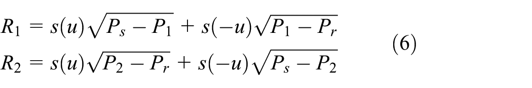
where β_e is the effective oil bulk modulus; V₀₁ and V₀₂ are the initial volumes of the two chambers, respectively; C_t is the coefficient of the total internal leakage of the actuator; Q₁ is the supplied flow rate to the forward chamber; and Q₂ is the return flow rate of the return chamber. Q₁ and Q₂ are related to the spool valve displacement of the servo valve, x_v, by ¹¹

$$\begin{array}{c}{Q}_1=k_q{x}_v[s\left(x_v\right)\sqrt{P_s-P_1}+s(-x_v)\sqrt{P_1-P_r}]\hfill \\ Q_2=k_q{x}_v[s\left(x_v\right)\sqrt{P_2-P_r}+s(-x_v)\sqrt{P_s-P_2}]\hfill \end{array}$$

(3)

where $k_q=C_{d}w\sqrt{2/\rho }$ and s(x_v) is defined as

$$s\left(x_v\right)=\{\begin{array}{c}1,\mathrm{if}{x}_v\ge 0\hfill \\ \multicolumn{1}{c}{0,\mathrm{if}{x}_v<0}\end{array}$$

(4)

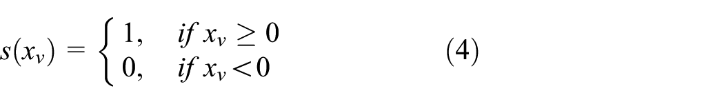
where k_q is the valve discharge gain, C_d is the discharge coefficient, w is the spool valve area gradient, ρ is the density of oil, P_s is the supply pressure of the fluid, and P_r is the return pressure.

In this article, it is assumed that the control applied to the servo valve is directly proportional to the spool position, then the following equation is given by x_v = k_iu, where k_i is a positive electrical constant and u is the input voltage. ¹¹ Then, from equation (4), s(x_v) = s(u).

Therefore equation (3) can be transformed to

$$\begin{array}{c}{Q}_1=g{R}_{1}u\hfill \\ Q_2=g{R}_{2}u\hfill \end{array}$$

(5)

where g = k_qk_i and

$$\begin{array}{c}{R}_1=s\left(u\right)\sqrt{P_s-P_1}+s(-u)\sqrt{P_1-P_r}\hfill \\ R_2=s\left(u\right)\sqrt{P_2-P_r}+s(-u)\sqrt{P_s-P_2}\hfill \end{array}$$

(6)

Assumption 1

In practical hydraulic system under normal working conditions, both P₁ and P₂ are bounded by P_r and P_s, ¹⁰ that is, 0 < P_r < P₁ < P_s and 0< P_r< P₂ < P_s.

Based on equations (1), (2), and (5), define x = [x₁, x₂, x₃] ^T  = [y, $\stackrel{·}{y}$ , A₁P₁ − A₂P₂] ^T as the system states. Thus, the entire system can be expressed in a state–space form as

$$\begin{array}{c}{\stackrel{·}{x}}_1=x_2\hfill \\ m{\stackrel{·}{x}}_2=x_3-B{x}_2-A_f{S}_f\left(x_2\right)-d_n-\tilde{d}(x_1,x_2,t)\hfill \\ {\stackrel{·}{x}}_3=(\frac{A_1}{V_1}{R}_1+\frac{A_2}{V_2}{R}_2)g{\beta }_{e}u-(\frac{A_1^2}{V_1}+\frac{A_2^2}{V_2}){\beta }_e{x}_2\hfill \\ -(\frac{A_1}{V_1}+\frac{A_2}{V_2}){\beta }_e{C}_t{P}_L\hfill \end{array}$$

(7)

where d_n represents the lumped nominal value of the unmodeled dynamics and external disturbances, ²⁰ $\tilde{d}(x_1,x_2,t)=f(x_1,x_2,t)-d_n$ .

In general, the system is subjected to structured uncertainties due to large variations in system parameters m, B, A_f, V₀₁, V₀₂, g, β_e, C_t, and so on. In addition, $\tilde{d}(x_1,x_2,t)$ is clearly the system unstructured uncertainty which cannot be modeled by an explicit function. For simplicity, we only consider the system parameters B, A_f, d_n, C_t, which are difficult to learn, as the parametric uncertainties, and others are all known. Define the unknown but constant parameter set θ  = [θ₁, θ₂, θ₃, θ₄] ^T  = [B, A_f, d_n, C_t] ^T . Then, equation (7) can be transformed to

$$\begin{array}{c}{\stackrel{·}{x}}_1=x_2\hfill \\ m{\stackrel{·}{x}}_2=x_3-{\theta }_1{x}_2-{\theta }_2{S}_f\left(x_2\right)-{\theta }_3-\tilde{d}\hfill \\ {\stackrel{·}{x}}_3=g_{3}u-f_c-{\theta }_4{f}_u\hfill \end{array}$$

(8)

where

$$\begin{array}{c}{g}_3=(\frac{A_1}{V_1}{R}_1+\frac{A_2}{V_2}{R}_2)g{\beta }_e\hfill \\ f_c=(\frac{A_1^2}{V_1}+\frac{A_2^2}{V_2}){\beta }_e{x}_2\hfill \\ f_u=(\frac{A_1}{V_1}+\frac{A_2}{V_2}){\beta }_e{P}_L\hfill \end{array}$$

(9)

Assumption 2

Parametric uncertainties θ and uncertain nonlinearities $\tilde{d}$ satisfy

$$\begin{array}{c}\mathit{\theta }\in {\Omega }_{\mathit{\theta }}=\{\mathit{\theta }:{\mathit{\theta }}_{\mathbf{min}}\le \mathit{\theta }\le {\mathit{\theta }}_{\mathbf{max}}\}\hfill \\ \left|\tilde{d}(x_1,x_2,t)\right|\le {\delta }_d\hfill \end{array}$$

(10)

where θ _min  = [θ_1min, …, θ_4min] ^T ; θ _max  = [θ_1max, …, θ_4max] ^T ; and δ_d is a known function.

Assumption 3

The desired position y_d(t)=x_1d(t) is C³ continuous and bounded.

RBF NN-based adaptive robust nonlinear feedback controller design

Discontinuous projection mapping

Define $\tilde{\mathit{\theta }}=\hat{\mathit{\theta }}-\mathit{\theta }$ as the estimation error, where $\hat{\mathit{\theta }}$ denotes the estimation of θ . A discontinuous projection is defined as ⁹

$$\mathrm{Pro}{\mathrm{j}}_{{\hat{\theta }}_i}\left({•}_i\right)=\{\begin{array}{c}0,\mathrm{if}{\hat{\theta }}_i={\theta }_{i\max }\mathrm{and}{•}_i>0\hfill \\ \multicolumn{1}{c}{0,\mathrm{if}{\hat{\theta }}_i={\theta }_{i\min }\mathrm{and}{•}_i<0}\\ \multicolumn{1}{c}{{•}_i,\mathrm{otherwise}}\end{array}$$

(11)

where i = 1, 2, 3, 4. In equation (11), ${•}_i$ represents the ith component of the $\mathrm{vector}•$ , and the operation “<” for two vectors is performed in terms of the corresponding elements of the vectors. Suppose that θ is estimated using the following projection-type adaptation law

$$\stackrel{·}{\hat{\mathit{\theta }}}=\mathrm{Pro}{\mathrm{j}}_{\hat{\mathit{\theta }}}\left({\mathbf{\Gamma }}_1{\mathbf{\tau }}_1\right)\hat{\mathit{\theta }}\left(0\right)\in {\Omega }_{\mathit{\theta }}$$

(12)

where $\mathrm{Pro}{\mathrm{j}}_{\hat{\theta }}(•)=[\mathrm{Pro}{\mathrm{j}}_{{\hat{\theta }}_1}({•}_1),\dots ,\mathrm{Pro}{\mathrm{j}}_{{\hat{\theta }}_4}({•}_4){]}^T$ ; Γ₁ > 0 is a positive diagonal matrix, which denotes the parameter adaptation gain; and τ ₁ is an adaptation function to be synthesized in the controller design later. It can be shown that for any adaptation function τ ₁ , the above projection mapping has the following properties ²¹

$$\begin{array}{l}\left(P1\right)\widehat{\mathit{\theta }}\in {\Omega }_{\widehat{\theta }}=\{\widehat{\mathit{\theta }}:{\mathit{\theta }}_{min]}\le \widehat{\mathit{\theta }}\le {\mathit{\theta }}_{max}\}\\ \left(P2\right){\tilde{\mathit{\theta }}}^{\mathrm{T}}\left({\Gamma }_1^{-1}{\mathrm{Proj}}_{\widehat{\mathit{\theta }}}\left({\Gamma }_1{\tau }_1\right)-{\tau }_1\right)\le 0\end{array}$$

(13)

Controller design

Step 1

Noting that the first equation of equation (8) does not have any uncertainties, we can design in one step by combining the first two equations of equation (8). By introducing x_2eq as the virtual control input for x₂, we can define the following error variables

$$\begin{array}{c}{z}_1=x_1-x_{1d}\hfill \\ z_2={\stackrel{·}{z}}_1+k_1{z}_1=x_2-x_{2\mathrm{eq}},x_{2\mathrm{eq}}={\stackrel{·}{x}}_{1d}-k_1{z}_1\hfill \end{array}$$

(14)

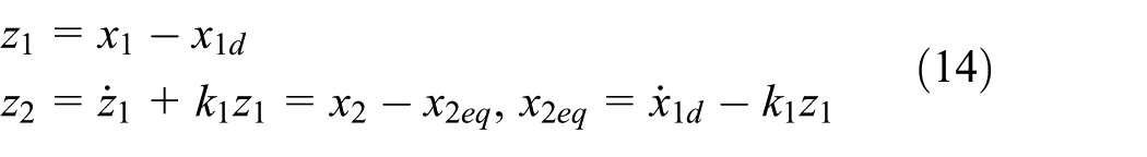
where k₁ is a positive feedback gain and z₁ denotes the position tracking error. Since z₁(s) = G(s)z₂(s), G(s) = 1/(s + k₁) is a stable transfer function, making z₁ converge to zero is equivalent to making z₂ converge to zero. Thus, the rest of the design is aimed to make z₂ converge to zero. Now according to equations (8) and (14), we have

$$\begin{array}{l}m{\stackrel{.}{z}}_2=m{\stackrel{.}{x}}_2-m{\stackrel{.}{x}}_{2eq}=x_3-{\theta }_1{x}_2\\ -{\theta }_2{S}_f\left(x_2\right)-{\theta }_3-\tilde{d}-m{\stackrel{.}{x}}_{2eq}\end{array}$$

(15)

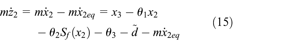
Step 2

In this step, we consider x₃ as the virtual control input and construct a control function α₂ for x₃ such that z₂ converges to zero, in which the transient performance is also guaranteed. The control function α₂ is given by

$$\begin{array}{c}{\alpha }_2={\alpha }_{2a}+{\alpha }_{2s}\hfill \\ {\alpha }_{2a}=m{\stackrel{·}{x}}_{2\mathrm{eq}}+{\hat{\theta }}_1{x}_2+{\hat{\theta }}_2{S}_f\left(x_2\right)+{\hat{\theta }}_3+\hat{\tilde{d}}\hfill \\ {\alpha }_{2s}={\alpha }_{2s1}+{\alpha }_{2s2},{\alpha }_{2s1}=-k_{2s1}{z}_2\hfill \end{array}$$

(16)

where k_2s1 > 0 is a feedback gain and $\hat{\tilde{d}}$ is the approximation of $\tilde{d}$ . In equation (16), α_2a is the model feedforward compensation term through online parameter adaptation given by equation (12), α_2s1 is the linear robust feedback term to stabilize the system nominal model by adjusting k_2s1, and α_2s2 is the nonlinear robust feedback term to be synthesized later. ²²

Now, we need to design an approximator to approximate uncertain nonlinearities such as $\tilde{d}$ and design α_2s2 to weaken simultaneously the parameter estimation error and uncertainty approximation error to stabilize the system. The two aspects of design processes are, respectively, as follows:

• 1. Given a sufficient number of hidden layer neurons and input information, the input–output mapping of RBF NN can be expressed as ²³ (structure chart is shown in Figure 2)

$$\tilde{d}={{\mathit{W}}^{*}}^T\mathit{h}\left(\mathit{x}\right)+{\epsilon }_{\mathrm{approx}}$$

(17)

$$h_j\left(\mathit{x}\right)=\exp (-\frac{{\Vert \mathit{x}-{\mathit{c}}_j\Vert }^2}{2b_j^2})$$

(18)

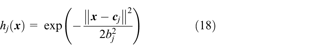
where x is the input of RBF network; h ( x ) = [h_j( x )]^T is Gaussian RBF, where j denotes the jth node of the hidden layer; W^* is the ideal weight of RBF network; and ε_approx is the approximation error of RBF network, which satisfies, respectively

$$\begin{array}{c}{\mathit{W}}^{*}\in {\Omega }_{W*}=\{{\mathit{W}}^{*}:{\mathit{W}}_{\mathbf{min}}^{*}\le {\mathit{W}}^{*}\le {\mathit{W}}_{\mathbf{max}}^{*}\}\hfill \\ \left|{\epsilon }_{\mathrm{approx}}\right|\le {\epsilon }_N\hfill \end{array}$$

(19)

Figure 2.

Structure of RBF neural network.

Take x  = [x₁, x₂] ^T as the input of the network, then the actual output through online learning is

$$\hat{\tilde{d}}={\hat{\mathit{W}}}^T\mathit{h}\left(\mathit{x}\right)$$

(20)

where $\hat{\mathit{W}}$ denotes the estimation of W ^*.

The weight adaptation law is given by

$$\stackrel{·}{\hat{\mathit{W}}}=\mathrm{Pro}{\mathrm{j}}_{\hat{W}}\left({\mathbf{\Gamma }}_2{\mathbf{\tau }}_2\right)$$

(21)

where $\mathrm{Pro}{\mathrm{j}}_{\hat{W}}(•)$ has the same form as $\mathrm{Pro}{\mathrm{j}}_{\hat{\theta }}(•)$ , Γ₂ denotes the weight adaptation velocity matrix, and τ ₂ is an adaptation function to be designed later.

Define z₃ = x₃ − α₂ as the input discrepancy, and by substituting equation (16) into equation (15), we have

$$m{\stackrel{·}{z}}_2=z_3-k_{2s1}{z}_2+{\alpha }_{2s2}-{{\phi }_2}^T\tilde{\theta }+{\tilde{W}}^{T}h\left(x\right)-{\epsilon }_{\mathrm{approx}}$$

(22)

where $\tilde{\mathit{W}}=\hat{\mathit{W}}-{\mathit{W}}^{*}$ denotes the estimation error of weights

$${\phi }_2={[-x_2,-S_f\left(x_2\right),-1,0]}^T$$

(23)

is the regressor for parameter adaptation. ⁹

• 2. α_2s2, as a robust control law, is designed to dominate the model uncertainties existed in the practical system, such as $\tilde{\theta }$ , $\tilde{W}$ , and ε_approx.

Noting assumption 2, equation (19), and P1 in equation (13), there exists α_2s2 such that the following two conditions are satisfied ³

$$z_2{\alpha }_{2s2}\le 0$$

(24)

$$z_2[{\alpha }_{2s2}-{\phi }_2^T\tilde{\theta }+{\tilde{W}}^{T}h\left(x\right)-{\epsilon }_{\mathrm{approx}}]\le {\epsilon }_2$$

(25)

where ε₂ is a positive design parameter which can be arbitrarily small. ²⁴

Here gives an example to choose α_2s2 to satisfy constraints such as equations (24) and (25)

$${\alpha }_{2s2}=-k_{2s2}{z}_2=-\frac{h_2^2}{4{\epsilon }_2}{z}_2$$

(26)

where k_2s2 is a positive nonlinear gain and h₂ represents the sum of the upper bounds of all errors, which means

$$|{\phi }_2^T\tilde{\theta }+{\tilde{\mathit{W}}}^{T}h\left(x\right)+{\epsilon }_{\mathrm{approx}}|\le h_2$$

(27)

Step 3

This step is to synthesize an actual control law for u such that z₃ converges to zero. Noting the third equation of equation (8), we have

$${\stackrel{·}{z}}_3={\stackrel{·}{x}}_3-{\stackrel{·}{\alpha }}_2=g_{3}u-f_c-{\theta }_4{f}_u-{\stackrel{·}{\alpha }}_2$$

(28)

where

$$\begin{array}{c}{\stackrel{·}{\alpha }}_2={\stackrel{·}{\alpha }}_{2c}-{\stackrel{·}{\alpha }}_{2u}\hfill \\ {\stackrel{·}{\alpha }}_{2c}=\frac{\partial {\alpha }_2}{\partial t}+\frac{\partial {\alpha }_2}{\partial x_1}{x}_2+\frac{\partial {\alpha }_2}{\partial x_2}{\widehat{\stackrel{·}{x}}}_2+\frac{\partial {\alpha }_2}{\partial \hat{\theta }}\stackrel{·}{\hat{\theta }}+\frac{\partial {\alpha }_2}{\partial \hat{W}}\stackrel{·}{\hat{W}}\hfill \\ {\stackrel{·}{\alpha }}_{2u}=\frac{\partial {\alpha }_2}{\partial x_2}{\widetilde{\stackrel{·}{x}}}_2\hfill \\ {\widehat{\stackrel{·}{x}}}_2=\frac{1}{m}(x_3-{\hat{\theta }}_1{x}_2-{\hat{\theta }}_2{S}_f\left(x_2\right)-{\hat{\theta }}_3-\hat{\tilde{d}})\hfill \\ {\widetilde{\stackrel{·}{x}}}_2=\frac{1}{m}({\phi }_2^T\tilde{\theta }-{\tilde{W}}^{T}h\left(x\right)+{\epsilon }_{\mathrm{approx}})\hfill \end{array}$$

(29)

where ${\stackrel{·}{\alpha }}_{2c}$ denotes the calculable part of ${\stackrel{·}{\alpha }}_2$ and can be used in the design of the actual controller u and ${\stackrel{·}{\alpha }}_{2u}$ is the incalculable part due to uncertainties which can be attenuated by the robust controller.

According to equations (28) and (29), the adaptive robust controller u is given by

$$\begin{array}{c}u=u_a+u_s\hfill \\ u_a=\frac{1}{g_3}(f_c+{\hat{\theta }}_4{f}_u+{\stackrel{·}{\alpha }}_{2c})\hfill \\ u_s=\frac{1}{g_3}(u_{s1}+u_{s2}),u_{s1}=-k_{3s1}{z}_3\hfill \end{array}$$

(30)

where k_3s1 > 0 is a feedback gain, u_a functions as an adaptive control law, and u_s as a robust control law. By substituting equation (30) into equation (28), we have

$$\begin{array}{cc}\multicolumn{1}{c}{{\stackrel{·}{z}}_3}& =-k_{3s1}{z}_3+u_{s2}+{\tilde{\theta }}_4{f}_u+{\stackrel{·}{\alpha }}_{2u}\hfill \\ \multicolumn{1}{c}{}& =-k_{3s1}{z}_3+u_{s2}+{\tilde{\theta }}_4{f}_u-\frac{\partial {\alpha }_2}{\partial x_2}\frac{1}{m}{\tilde{\theta }}_1{x}_2-\frac{\partial {\alpha }_2}{\partial x_2}\frac{1}{m}{\tilde{\theta }}_2{S}_f\left(x_2\right)\hfill \\ \multicolumn{1}{c}{}& -\frac{\partial {\alpha }_2}{\partial x_2}\frac{1}{m}{\tilde{\theta }}_3-\frac{\partial {\alpha }_2}{\partial x_2}\frac{1}{m}({\tilde{W}}^{T}h\left(x\right)-{\epsilon }_{\mathrm{approx}})\hfill \\ \multicolumn{1}{c}{}& =-k_{3s1}{z}_3+u_{s2}-{\phi }_3^T\tilde{\theta }-\frac{\partial {\alpha }_2}{\partial x_2}\frac{1}{m}({\tilde{W}}^{T}h\left(x\right)-{\epsilon }_{\mathrm{approx}})\hfill \end{array}$$

(31)

where

$${\phi }_3=\frac{1}{m}{[\frac{\partial {\alpha }_2}{\partial x_2}{x}_2,\frac{\partial {\alpha }_2}{\partial x_2}{S}_f\left(x_2\right),\frac{\partial {\alpha }_2}{\partial x_2},-m{f}_u]}^T$$

(32)

Similarly, one u_s2 can be selected to satisfy the following two conditions ³

$$z_3{u}_{s2}\le 0$$

(33)

$$z_3[u_{s2}-{\phi }_3^T\tilde{\theta }-\frac{\partial {\alpha }_2}{\partial x_2}\frac{1}{m}({\tilde{W}}^{T}h\left(x\right)-{\epsilon }_{\mathrm{approx}})]\le {\epsilon }_3$$

(34)

where ε₃ is a positive design parameter which can be arbitrarily small.

Taking the design solution of α_2s2 for reference, one feasible example of u_s2 is given below

$$u_{s2}=-k_{3s2}{z}_3=-\frac{{h_3}^2}{4{\epsilon }_3}{z}_3$$

(35)

where k_3s2 is a positive nonlinear gain and

$$|{\phi }_3^T\tilde{\theta }+\frac{\partial {\alpha }_2}{\partial x_2}\frac{1}{m}({\tilde{W}}^{T}h\left(x\right)+{\epsilon }_{\mathrm{approx}})|\le h_3$$

(36)

Main results

Theorem 1

For any adaptation function τ ₁ and τ ₂ , the designed adaptive robust controller (30) has the following properties:

All signals in the closed-loop controller are bounded, and consider the Lyapunov function $V_3=(1/2)k_1^2{z}_1^2+(1/2){\mathrm{mz}}_2^2+(1/2)z_3^2$ which is bounded by

$$V_3\le e^{-\mu t}{V}_3\left(0\right)+\frac{\epsilon }{\mu }\left[1-e^{-\mu t}\right]$$

(37)

where $\epsilon ={\epsilon }_2+{\epsilon }_3$ , $\mu \stackrel{\Delta }{=}2{\lambda }_{\min }({\Lambda }_3)\min \{1/k_1^2,1/m,1\}$ , and ${\lambda }_{\min }({\Lambda }_3)$ is the minimum eigenvalue of the positive definite matrix Λ₃ which is given by

$${\Lambda }_3=\left[\begin{array}{ccc}{k}_1^3\hfill & -\frac{k_1^2}{2}\hfill & 0\hfill \\ \multicolumn{1}{c}{-\frac{k_1^2}{2}}& k_{2s1}\hfill & -\frac{1}{2}\hfill \\ \multicolumn{1}{c}{0}& -\frac{1}{2}\hfill & k_{3s1}\hfill \end{array}\right]$$

(38)

Theorem 2

With the discontinuous projection-type parameter adaptation law (12) and weight adaptation law (21) in which τ ₁ and τ ₂ are chosen, respectively, as

$${\mathit{\tau }}_1={\mathit{\phi }}_2{z}_2+{\mathit{\phi }}_3{z}_3$$

(39)

$${\mathit{\tau }}_2=(\frac{\partial {\alpha }_2}{\partial x_2}\frac{1}{m}{z}_3-z_2)\mathit{h}\left(\mathit{x}\right)$$

(40)

then the control input (30) guarantees.

If after a finite time, the system is subjected to parametric uncertainties only with RBF network–based ARC law (30) (i.e. $\tilde{d}={{\mathit{W}}^{*}}^T\mathit{h}(\mathit{x})$ , ²⁵ namely, ε_approx = 0 after a finite time), in addition to results in theorem 1, asymptotic output tracking is also achieved, ⁹ that is, z  → 0 as t → ∞, in which z  = [z₁, z₂, z₃] ^T .

Proof

See Appendix 1.

Remark

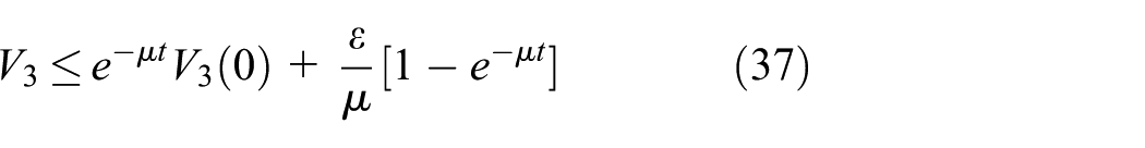
From theorem 1, some theoretical results imply that the control strategy proposed can obtain an expected transient performance in the form of exponential convergence and the final steady-state performance is also able to be guaranteed by adjusting certain controller parameters freely in a specified form. It is particularly important to have such desired transient performance and final tracking precision, which are always the target of high-accuracy motion control systems. Results achieved from theorem 2 reveal that, by way of utilizing parameter and weight adaptation laws, the parametric uncertainties may be restrained, and an enhanced steady performance is obtained to guarantee the stabilization of hydraulic servo systems.

Simulation results

To verify the performance of the proposed RBF NN-based adaptive robust controller (ARCNN), computer simulation has been carried out. The results are compared with those obtained from an adaptive robust controller and a proportional–integral–derivative (PID) controller. The three controllers are tested for a sinusoidal-like motion trajectory x_1d = sint[1 − exp(−0.01t ³ )], and four cases are tested for this motion trajectory.

Case 1: normal case

Assuming no any disturbances from the external environment exist, by calculating the control input u under the integration of multiple control policies proposed, take the control input u into account, which is directly implemented to the practical system.

Case 2: input disturbance case

By transforming the control input u into 0.5u, which indicates the input disturbance be loaded to the practical system. So as to suppress strong structured uncertainties, this type of disturbance is applied, on one hand, which will product great influences on the rate of parameter/weight convergence and, on the other hand, which is used to examine the adaptive capacity of the proposed controller against input disturbances and the final tracking performance of control systems.

Case 3: position–velocity disturbance case

As the name suggests, by exerting influences of the position x₁ and the velocity x₂ on the practical motion system, multiple disturbances integrated are applied by modifying the control input u as u − 0.5x₁x₂. Exposed to heavy unstructured uncertainties, the performance of system itself will bring about great changes, especially affecting $\tilde{d}$ greatly under this type of disturbance.

Case 4: position–velocity–input disturbance case

By synthesizing case 2 and case 3, the worst working condition is implemented to the practical physical system via loading 0.5u − 0.5x₁x₂ as the control input. Similarly, this compound disturbance will exert great influences on the convergence of parameters and weights, together with $\tilde{d}$ . Whether the proposed controller achieves a stable performance under this case or not, it can be viewed as the most comprehensive verification among all cases.

To illustrate the controller design, simulation results are obtained for the dynamic models of the hydraulic system discussed in section “Problem formulation and dynamic models,” with the following actual parameters: P_s = 7 × 10⁶ Pa, P_r = 0 Pa, V₀₁ = V₀₂ = 1 × 10⁻³ m³, A₁ = A₂ = 2 × 10⁻⁴ m², m = 40 kg, B = 80 N s/m, C_t = 7 × 10⁻¹² m⁵/(N s), g = 4 × 10⁻⁸ m⁴/(s V √N), β_e = 2 × 10⁸ Pa, A_f = 10 N, $S_f=2\arctan (1000\stackrel{·}{y})/\pi$ , and d_n = 0 N. Thus, the actual value of θ is θ = [80 10 0 7 × 10⁻¹²] ^T , and the uncertain nonlinearity term $\tilde{d}=0$ . The controller parameters are given, respectively, under the compared three controllers.

ARCNN

The control gains are chosen as k₁ = 250, k₂ = k_2s1 + k_2s2 = 100, and k₃ = k_3s1 + k_3s2 = 50. The bounds of parametric ranges are given by θ _min  = [60 −20 −50 4 × 10⁻¹²] ^T and θ _max  = [100 20 50 10 × 10⁻¹²] ^T . The initial estimation of θ and W are $\hat{\mathit{\theta }}(0)=[\begin{array}{cccccc}60\hfill & 0\hfill & 0\hfill & 4\hfill & 10\hfill & 12\hfill \end{array}{]}^T$ and $\hat{\mathit{W}}(0)=[\begin{array}{ccccc}-10\hfill & -10\hfill & -10\hfill & -10\hfill & -10\hfill \end{array}{]}^T$ , respectively. The parameter adaptation rates are set as Γ₁ = diag{50 20 1 × 10⁻¹⁵ 1 × 10⁻¹⁰} and the weight adaptation rates as Γ₂ = diag{10 10 10 10 10}. Parameters of RBF NN are chosen as c  = [−0.8 −0.4 0 0.4 0.8] ^T and b  = [5 5 5 5 5] ^T .

ARC

The control gains are chosen as k₁ = 100, k₂ = 80, and k₃ = 50. The parameter adaptation rates are set as Γ₁ = diag{100 30 50 1 × 10⁻³⁰}. The other controller parameters are the same as the corresponding parameters in ARCNN.

PID

PID controller, which is generally acted as a reference controller for comparison, is commonly treated as a feedback-loop part in industrial control applications. Via an error-and-try mechanism, its control gains, which are chosen as k_p = 200, k_i = 0, and k_d = 50, can be tuned carefully to maintain the stability of the system.

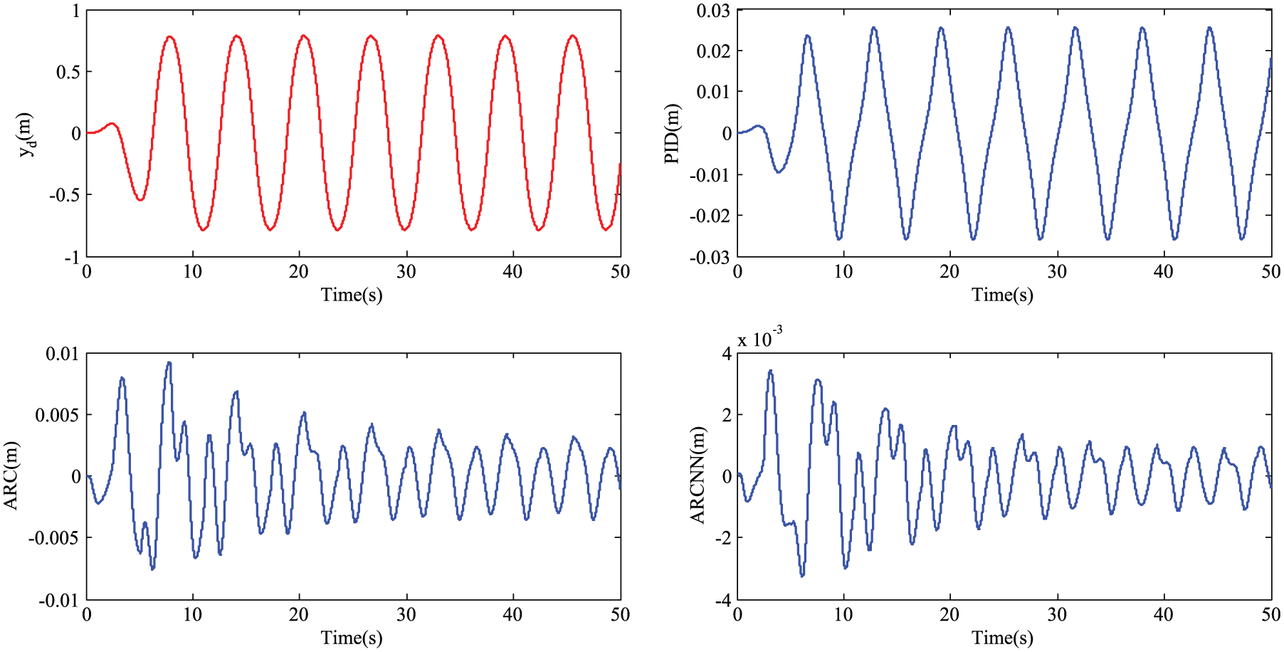
The desired motion trajectory and corresponding tracking performance under the three controllers in normal case are shown in Figure 3. According to this figure, we can conclude that the proposed ARCNN and ARC controllers have better transient and final tracking performance than the PID controller, which proves that employing ARC can estimate parameter uncertainties and compensate them in controllers. The PID controller just has some robustness against uncertainties, and its tracking error (about 0.013 m) is relatively large. Although ARC has some learning capability via parameter adaptation, the learning process makes no difference to uncertain nonlinearities (i.e. $\tilde{d}$ ). That is why the performance of ARC is worse than that of the controller with RBF. In addition to estimate uncertain parameters (parameter estimation is shown in Figure 4), the ARCNN controller can simultaneously overcome structured and unstructured uncertainties with RBF NN, which greatly improves the tracking performance. This verifies the effectiveness of the proposed scheme with ARC and RBF NN. From Figure 1, the final tracking error of ARCNN is reduced down to 2.6 × 10⁻⁴ m, while ARC has a larger tracking error (about 3.7 × 10⁻⁴ m).

Figure 3.

Tracking errors of the three controllers in normal case.

Figure 4.

Parameter estimation in normal case.

To examine the effectiveness of the proposed algorithm against structured uncertainties, the simulation under the input disturbance case is implemented with the same desired motion trajectory. The tracking errors of the three controllers are shown in Figure 5. In this case, the performance of ARC and ARCNN is much better than that of PID, whose tracking error (about 0.026 m) is greatly increased. The input disturbance, namely, structured uncertainties, can be captured by the adaptation law of ARCNN, and the residual disturbances can be compensated by RBF NN. From the fourth figure, we can obtain that the maximal steady tracking error (about 3 × 10⁻⁴ m) in ARCNN appears to be no much more different than that under normal case, which can also verify the effectiveness of the proposed controller with the combination of ARC and RBF NN.

Figure 5.

Tracking errors of the three controllers in input disturbance case.

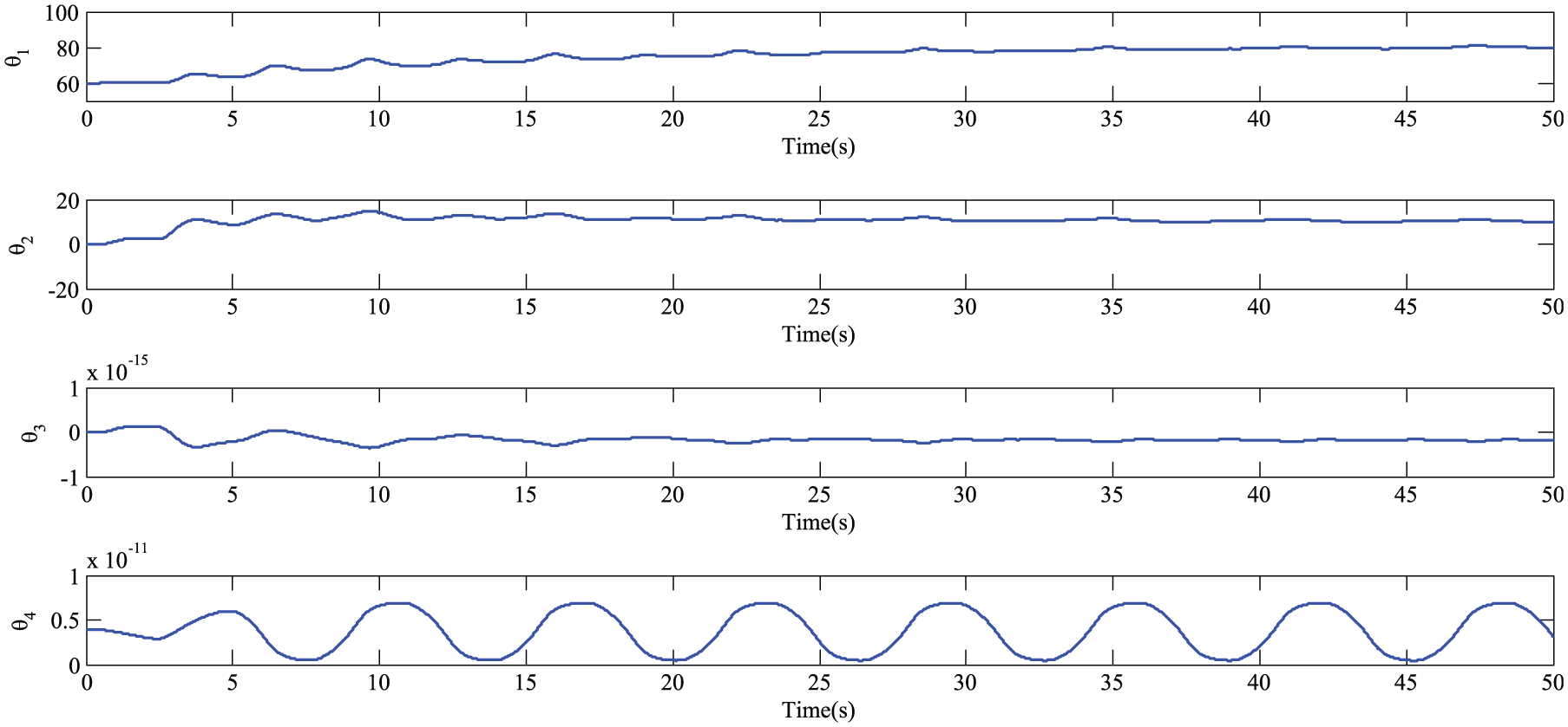
To further examine the robustness of the proposed algorithm against unstructured uncertainties, the position–velocity disturbance case is taken into consideration, which will be the dominant factor affecting the tracking performance. The tracking errors of the three controllers are shown in Figure 6. As seen from this figure, although faced with heavy unstructured uncertainties, the proposed ARCNN controller (maximal steady error of about 5 × 10⁻⁴ m) is also able to weaken unexpected effects and achieves the best tracking performance among all three controllers. The parameter estimation is presented in Figure 7. The estimation process of θ in ARCNN is unstable since the driving force of its parameter estimation is small; simultaneously, disturbed by this unstructured disturbance (disturbance and its estimation is shown in Figure 8), its learning capability is partially receded. In addition, the ARC controller exhibits worse performance than that shown previously due to the large position–velocity disturbance (maximal steady error of about 1.5 × 10⁻³ m).

Figure 6.

Tracking errors of the three controllers in position–velocity disturbance case.

Figure 7.

Parameter estimation in position–velocity disturbance case.

Figure 8.

Disturbance and its estimation in position–velocity disturbance case.

To farthest consider the authentic complex working conditions, the position–velocity–input disturbance is employed to examine the performance of the proposed controller. In this case, mixed with structured and unstructured uncertainties, all three controllers are affected at some extent. The tracking performance under this disturbance is shown in Figure 9. As seen, while there exists oscillation in the initial phase, the proposed ARCNN controller still achieves the satisfied tracking performance with a maximal steady tracking error of about 1 × 10⁻³ m. It greatly proves the effectiveness of the proposed algorithm with RBF NN. Nevertheless, ARC has slightly insufficient abilities to deal with this severe disturbance very well and present the large tracking error (about 3.5 × 10⁻³ m).

Figure 9.

Tracking errors of the three controllers in position–velocity–input disturbance case.

Conclusion

In this article, an integrated control strategy named an ARC with an RBF NN, which takes into consideration not only the parametric uncertainties but also the uncertain nonlinearities, has been put forward for a high-accuracy motion control system driven by a hydraulic actuator. Lyapunov stability theory, the tool which is used to provide performance guarantees of closed-loop systems, is a critical theoretical basis to analyze the stability of control systems. Extensive results obtained by simulation under four working conditions are used to testify the feasibility of the proposed control strategy, which indicates that by introducing an RBF NN-based disturbance observer to ARC, although strong external disturbances exist in actual systems, a desired transient tracking performance and the final tracking accuracy can also be guaranteed. By merging the fundamental working mechanisms of the two control approaches, it proves to achieve better performance results than that of the single ARC approach, particularly in facing parameter uncertainties and strong external disturbances, the design idea which inspires us to explore the more effective controller design scheme and propel it to industrial utility as soon as possible.