Sage Journals: Discover world-class research

Abstract

This article deals with the packing problem of irregular items allocated into a rectangular sheet to minimize the waste. Conventional solution is not visual during the packing process. It obtains a reasonable and relatively satisfactory solution between the nesting time and nesting solution. This article adopts a physical method that uses rubber band packing algorithm to simulate a rubber band wrapping those packing irregular items. The simulation shows a visual and fast packing process. The resultant rubber band force is applied in the packing items to translate, rotate, and slide them to make the area decrease and obtain a high packing density. An improved analogy QuickHull algorithm is presented to obtain extreme points of rubber band convex hull. An adaptive module could set a variable rubber band force and a variable time step to make a proper convergence and no intersection. A quick convex decomposition method is used to solve the problem of concave polygon. A plural vector expression approach is adopted to calculate the resultant vector of the rubber band force. Several cases are compared with the benchmark problems to prove rubber band packing algorithm performance.

Keywords

Packing problem irregular cutting stock visual rubber band packing algorithm physical method

Introduction

In several industrial applications, one is required to allocate a set of rectangular or irregular items to larger rectangular standardized stock units to minimize the waste, such as shipbuilding, textile, wood, plastic, sheet metal, and leather manufacturing.

The irregular packing problem is more complex than the rectangular one which has been shown to be nondeterministic polynomial time (NP) complete.¹ Many researchers have attempted to solve the nesting problem. A detailed survey by Bennell and Oliveira² presents a tutorial of current methods used by researchers in cutting and packing of irregular shapes. These heuristics, meta-heuristics, and hybrid algorithms have been impressively applied to this problem as powerful optimization tools. In above methods, no item is placed in the sheet in the initial state, while all of them are in the final state. It is difficult to watch the nesting result during the packing process directly, while just obtain a reasonable and relative satisfactory solution between the nesting time and nesting solution, and difficult to adjust the nesting result by hand with some requirement.

An irregular stock cutting system (NestRB) based on rubber band packing algorithm (RBPA) is developed on Visual C++ software, which aimed to build a visual intelligent system. This article includes a detailed description to its algorithm and flowchart.

The system described has the following features:

It is considerably fast, while producing solutions of high quality.

Unlike many existing packing algorithms, packing course of the present system is visual for user every step, showing perceptual intuition. This is especially important for industrial applications to show the result of the layout design.

In contrast to most published algorithm, the present algorithm described here is based on the method of physics, which is a new method to solve these problems.

This article is organized as follows: A brief review of previous work in the field is presented in section “Related works”; section “New approach for the nesting system” states the RBPA including its definition and flow diagram; in section “Some key problems of the NestRB system,” the key problems of the proposed system are described in detail; section “Experimental results” presents experimental results on benchmark problems from the literature that demonstrates the capabilities of the proposed system; and section “Conclusion” draws a conclusion.

Related works

To find an optimal solution for packing problem, the earliest solution was linear programming planning method which was suggested by Paull³ in 1950s last century to solve the rectangle packing problem in printing and paper industry, and the stock utilization is priced high.

Due to the problem of NP complete, the solution turns to some approximation method. Huang et al.⁴ used exhaustive search method to seek the minimal area enveloping rectangular of the sheet metal part. Xue et al.⁵ used genetic simulated annealing (SA) hybrid algorithm to seek the minimal area enveloping rectangular of convex polygon. Chaudhuri and Samal⁶ used a least-square approach to determine the directions of major and minor axes of the item to obtain the minimal area enveloping rectangular. It must be mentioned that minimal enveloping rectangular is an approximate value, which is not effective to improve the material utilization.

For good solution, most of the heuristics have been applied to nesting problems. Dagli⁷ proposed a heuristic algorithm based on pattern subset which was combined by fewer graphs. Oliveira et al.⁸ implemented a more sophisticated placement strategy called TOPOS approach which allows the layout to grow from a floating origin, and both the next polygon to be placed and its position are determined using a range of criteria. A detailed survey by Bennell and Oliveira² mentioned most heuristic methods.

Those algorithms solved some kinds of the stock cutting problem, but the feasibility is not good. In order to avoid local optima, most researchers attempt to find a solution of good quality (but not necessarily the optimal one) in reasonable computational times using evolutionary algorithms, hybrid algorithm, and other meta-heuristic methods.⁹ Gomes and Oliveira¹⁰ developed a hybrid algorithm which utilizes SA on guiding the search and linear programming models to carry out the local optimization of the resulting layouts during the search process. Hifi and M’Hallah¹¹ developed an approach which consists of a constructive heuristic and a hybrid genetic algorithm (GA)-based heuristic to solve the two-dimensional (2D) layout problem for the cases of regular and irregular shapes. Martins and Tsuzuki¹² proposed a heuristic based on SA for the problem of minimizing the waste while packing a set of items of irregular shape in a bin, in which rotation of the items is allowed.

In the literatures, we can find most approaches tried to tackle the different issues need to define the rule of the location. Dowsland et al.¹³ pointed out that the bottom-left (BL) placement strategy is the common policy to the 2D irregular packing problems. The results obtained using the proposed methodology are compared with those obtained using the BL placement strategy in combination with random search (RS). Burke et al.¹⁴ applied a BL-fill heuristic algorithm to allocate the items, and a number of techniques to resolve possible overlaps between the nested items have been introduced. Weng and Kuo¹⁵ developed an irregular stock cutting platform, using bitmap representation to transform all shapes drawn by AutoCAD and a BL-fill algorithm to arrange all shapes. Nielsen and Odgaard¹⁶ applied a meta-heuristic method called guided local search to the nesting problem, which given a set of items, we can find whether it can fit inside a given large object. The quality of their solutions is often close to the best solutions achieved for a variety of benchmark problems, but the execution time of their method is high.

The first obstacle researchers come up against is the geometry layout touch algorithm. While the most popular and most frequently cited geometry tool in the modern literature on the cutting and packing problems is the so-called no-fit polygon (NFP), which can compute the touch location and overlap judgment fast. Dowsland and Dowsland¹⁷ provided an irregular shape BL layout algorithm based on NFP. Liu and He¹⁸ proposed an NFP algorithm based on the lowest center of gravity. The center of the packed item’s gravity is located as low as the bottom, and the border is maintained to be horizontal after the item is packed into the metal plate to conveniently pack the latter part. But it does not ensure of the effectiveness of this squeeze’s method. Hopper⁹ elaborated the research of 2D irregular shape layout problem and used it to solve irregular shape layout problem together with GA. The instances he used make the packing items having admissible orientations with 0, 90, and 180.

NFP is usually used together with the intelligent search algorithm such as GA, SA, and so on to solve the layout problem, which is time-consuming. Utilizing NFPs, the polygon collision detection can be reduced to a significantly less expensive point inside polygon test. But NFP is applied to work only with polygonal objects without rotations or rotation limitation, which makes the solution not good enough. Liu and Ye¹⁹ proposed a heuristic algorithm based on the principle of minimum total potential energy which allows each item to have up to 32 orientations making the execution time reasonable.

The physical method that could be used to solve the packing problem is a novel concept proposed by Li and Milenkovic²⁰ and Fadel and Sinha.²¹ The former used a velocity-based model to solve the compaction problem but took a longer time because of recomputing velocities. The latter is used by Dong et al.²² to solve the three-dimensional (3D) space layout problem. This system adopts this physical method and improved it to construct a rubber band convex hull (rbCH) to solve cutting-stock problem on the rectangular sheet material. This method could tackle the free-rotation packing items which is also tackled by Stoyan et al.²³ Free-rotation items could obtain a pretty good solution.

New approach for the nesting system

The present system aims to place some irregular shapes together on the sheet material which may have fixed width and variable length called rectangular strip packing problem (RSPP) or some sheet with fixed width and fixed length called rectangular bin packing problem (RBPP), wasting as little resource material as possible and showing a visual intelligent packing simulation. RBPP problem is limited to some jigsaw puzzle created by us (see section “Some problems created by us”) which is simple, and the initial position is not a mess but just splits from the integrated puzzle.

Definition

RBPA is a physical analogy method which solves packing problems by simulating the physical movements of a set of items wrapped by a rubber band (see Figure 1). The analogy process can be described as follows: A rubber band is stretched around the items, and the elastic energy is considered high initially. The items are brought together to obtain a compact status because the stretched rubber band has the tendency to be lower energy until the resultant force is zero.

Figure 1.

Example of rubber band physical movement.

The system simulates this rubber band physical movement process to achieve a packing layout. For a given set Q = {Q₁,…, Q_n} of n items described as polygons and a bearing sheet C = {L, W}, where L (fixed or presetting) is the length of sheet and W is the width, the NestRB system requires all the items to be placed reasonably on the bearing sheet to meet the following technical requirements:

No interference between two items (Q_ij (X)) and no interference between the items and boundary of the sheet (C_i (X)), where variables X are the positions and orientations of the items

\sum_{i = 1}^{n} \sum_{j = 1}^{i - 1} Q_{ij} (X) + \sum_{i = 1}^{n} C_{i} (X) = 0

(1)

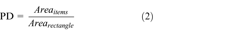
The ratio of the total area of all the packing items to the area of the rectangle sheet that encloses these items called packing density (PD)²⁴ should be as big as possible

PD = \frac{Are a_{items}}{Are a_{rectangle}}

(2)

RBPA

RBPA needs movement resolution to simulate the movement and the final compact status. Movement resolution is introduced as follows: Initially, the items wrapped by rubber band will translate to the center along the direction determined by the resultant elastic force (see Figure 2) until collision occurs; then, the items rotate around the contact points until the edges contact each other; at the same time, the items slide along the contact edge to make a further compact (see Figure 3). The movement of translation, rotation, and sliding iterates until no motion is possible to improve the compactness or resultant force of each item is zero.

Figure 2.

Resultant elastic force.

Figure 3.

Translation, rotation, sliding, and collision.

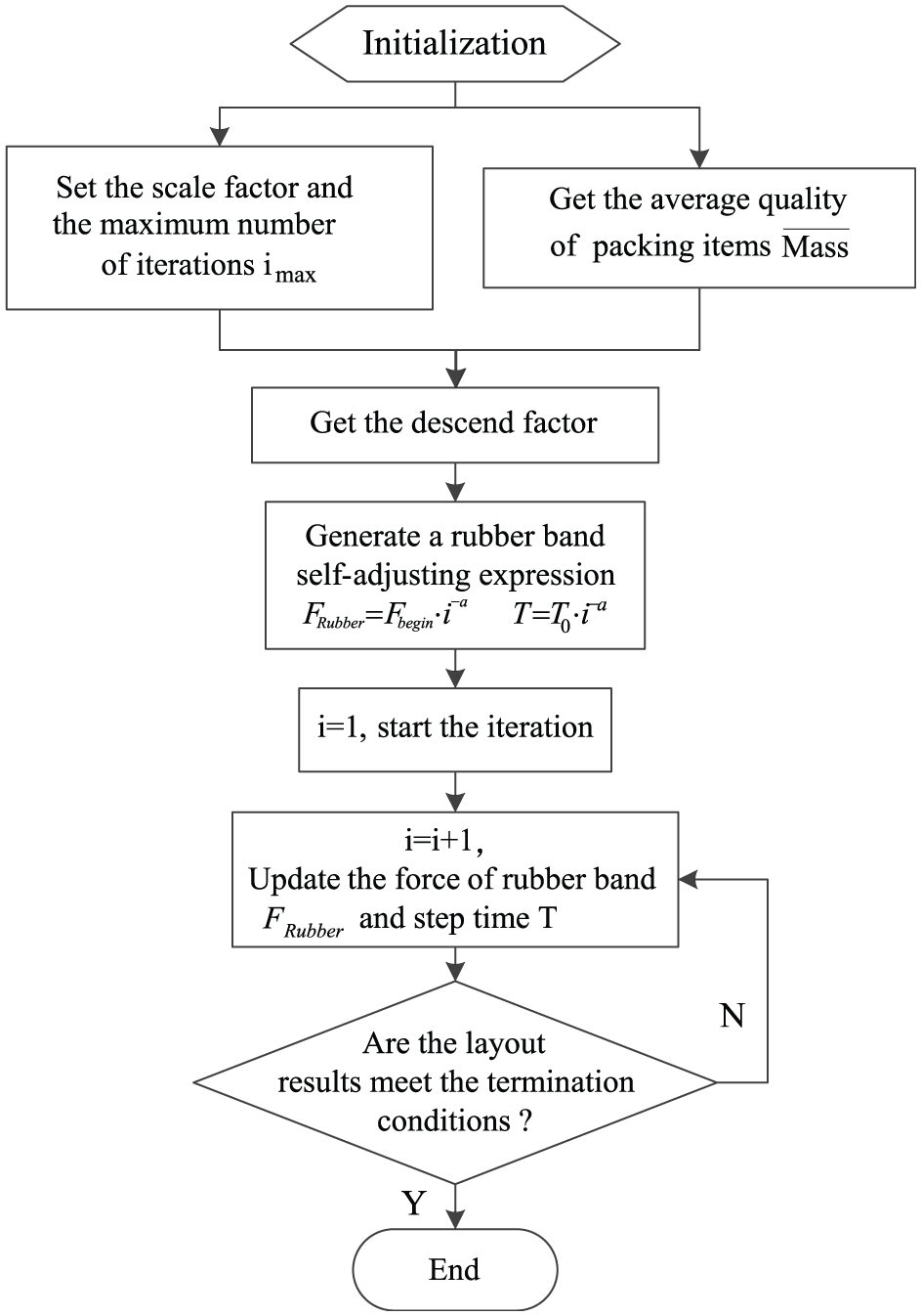
Figure 4 illustrates the detailed flow of our RBPA algorithm and shows the interaction between master procedure and adaptive module for elastic force F and time step T. According to this flowchart, if T is time step whose constant would be set smaller than the minimum time of human’s vision, a rough value of 1/60 s is recommended. Two times of tunnel detection and six times of collision detection will be executed within each time step. That is an empirical value to avoid intersection, full overlap, and traverse, as shown in Figure 5.

Figure 4.

Diagram of RBPA.

Figure 5.

Three types of collisions: (a) intersection, (b) overlap, and (c) tunnel.

But constant elastic force would lead to no divergence of result, and constant time step would lead to interference phenomenon that occurs during latter adjustment stage. Adaptive module could obtain proper initial rubber band force F_begin and T. The adaptive function is stated in section “Rubber band force and time step based on adaptive function.”

Improved RBPA for NestRB system

RBPA is not suitable for cutting-stock problem because it could not compact the items into a rectangle area (see Figure 1). RBPA should be improved for the NestRB system which has packed components on a rectangle sheet to avoid the RBPA obtaining a compact space similar to a circle. The process of the improved algorithm is presented in detail as follows:

Step 1: The exterior of the rectangle sheet is divided into four regions, and four boundaries are obtained as shown in Figure 6;

Step 2: The packing items are classified into four lists and arranged into these four regions randomly;

Step 3: Generate the vertex of the each item convex hull in each region. Find the farthest distance which is the vertexes apart from the center of rectangle. Make the farthest as the radius, and the four rbCHs are generated for these four regions. The algorithm process is stated in section “rbCH”;

Step 4: Length of rbCH shrinks along the boundary. The packed items would move to the rectangle region under the elastic force until each length of the rubber band is equal to the side length of the rectangle shell, respectively.

Figure 6.

Packing process demonstration of NestRB system.

Some key problems of the NestRB system

To realize a visual packing process and operation efficiency of the NestRB system based on this physical method, let us make four assumptions:

Assume no friction forces since only the positions of the objects are important;

The rubber band can be stretched indefinitely and elastic force is invariable in packing process;

The items are arranged in the system with no overlap;

Items will not bounce back, switch positions, or pass through each other when contact occurs during the packing process as shown in Figure 5.

In addition to the above assumptions, there are three key problems:

How to set rubber band force and time step;

Decomposition of concave polygon;

Geometry identification and resultant force.

Rubber band force and time step based on adaptive function

F is the rubber band force which has great influence on the efficiency of program and even leads to no divergence of result. F would be varied with the elongation of rubber band following the Hooke’s law and resolved in each iteration of the procedure. In the initial stage of the movement as shown in Figure 7(a), packing items are distributed far away from the center of layout space, long distance with each other, so that each item moves with a high moving speed. F would be set bigger than latter in favor of making the items gather to the center quickly, and the value would rapidly decrease to improve the efficiency of the early stage of the algorithm. While in the adjustment stages of movement as shown in Figure 7(b), each item no longer has a larger moving or just rotation. So, F would be maintained at a certain value, ensuring that it is enough to make a fine adjustment and convergence to the optimal solution at a reasonable speed.

Figure 7.

Rapid decrease with rubber band force: (a) initial stage, (b) adjustment stage, and (c) relation curve of power function.

Adaptive module in the diagram of RBPA as shown in Figure 4 can obtain a good F according to the current layout status. This article presents a self-adaptive algorithm based on power function (Figure 7(c)) to obtain a suitable rubber band force which can control the process of the layout rubber with a reasonable convergence rate and obtain a satisfactory result. Figure 7(c) shows the curve of power function (see formula (3)) when obtaining a different value α. This power function curve is divided into three main phases: decline phase, transition phase, and stable phase. In formula (3), x is an independent variable, and y is a dependent variable. If i (iteration times) replaces the x, the F_rubber replaces the y and add a coefficient F_begin, formula (4) would be deduced from formula (3). It can adjust function drop speed and the size of the stable phase function value by adjusting the parameters α. Our packing process could simulate these three phases. Figure 8 shows the flow diagram of rubber band adaptive module.

Figure 8.

Flow diagram of adaptive module for rubber band force.

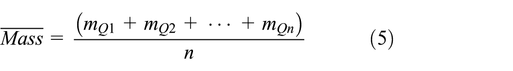
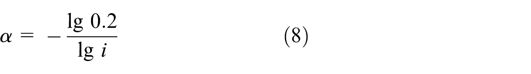
The α is a crucial value in Figure 9. Formula (4) expresses the rubber band force of ith iteration in algorithm, where i = 1, 2,…, n, denotes the iterative times. F_begin denotes the rubber band force at the beginning of the packing process. The α denotes the descending coefficient. Suppose F is equal at each side of rbCH. The force applied on each item would be equilibrium to avoid that large item being forced small while the small item being forced too little. The average of all items’ quality $\bar{Mass}$ (equation (5)) multiplied by the proportion coefficient K is thought of as the initial rubber band force F_begin (equation (6)). K could be set according to the experience through the software settings window, 1, 10, and 100 generally. The α would be set by the principle of 80/20 that is a law of least effort making 20% iteration of the total occupy of the main decline stage, while the remaining 80% is the transition stage. Suppose i_max = 100, where i_max is the largest number of iterations. Rubber band force would decline to 20% of the initial rubber band force at top 20% iteration rapidly. Rubber band force would change a little in the subsequent iteration until algorithm terminated. A proper value for α could be deduced from formulas (4) and (7)

y = x^{- α} (α > 0)

(3)

F_{Rubber} = F_{begin} \cdot i^{- α}

(4)

\bar{Mass} = \frac{(m_{Q 1} + m_{Q 2} + \dots + m_{Qn})}{n}

(5)

F_{begin} = k \cdot \bar{Mass}

(6)

F_{Rubber} = F_{begin} \cdot i^{- α} = F_{begin} \cdot 20 %

(7)

α = - \frac{\lg 0.2}{\lg i}

(8)

T = T_{0} \cdot i^{- α}

(9)

T_{0} = \frac{1}{60}

(10)

Figure 9.

Performance of layout with force based on adaptive function contrast to constant force.

The performance of the layout with force based on adaptive function contrast to constant force applied on rubber band at each step has been tested, which shows force adopted power function at each step making speed of convergence faster than the other, as shown in Figure 9.

If the distance between the packing items is small, and the constant time step mentioned in section “RBPA” is not enough, the intersection would occur. Time step is also set by the principle of 80/20 as mentioned above. The crucial factors of time step are its speed and distance between the packing items. However, calculating the distance between items involved in n items would increase the computational complexity. The ratio of current rbCH’s length surrounded at items with the minimum length denotes the elongation of the rubber band. The bigger the value, the greater the rubber band force, and the time step is larger. Due to the principle of 80/20 applied on the force to make a good performance, it is also applied on time step. That is to say, the farther the distance of items, the bigger the time step. The time step as shown in formula (9) could decline following F to obtain a proper value avoiding the intersection. The α denotes the descending coefficient set by formula (8) as same as F. T₀ denotes the initial time step at the first iteration of the packing process. It is given by formula (10) and could be set according to the experience through the software settings window, 1/60 generally.

Packing item geometry identification and data structure

Most widely used geometric representations for identifying geometries can be roughly classified into the bitmap (BMP-rep) and the vector (Vector-rep).¹⁶ For the packing process that needs to compute the resultant elastic force, the vector should be selected because it can record data of a geometric outline such as vertexes and edges to represent the geometry of the items and the component of the resultant force. Convex hull construction is used to represent the packing item convex hull (PiCH) and the rbCH wrapped by rubber band.

A 2D computer-aided design (CAD) software is often used to draw the packing item which is a file of dxf format. The first thing is to read and convert dxf file to PiCH when these items are put into NestRB system.

The dxf file is readable, and the construction has seven regions including HEADER, CLASSES, TABLES, BLOCKS, ENTITIES, OBJECTS, and ending of file (EOF). These regions are formed by records forming of group codes and data item successively. The system deals with the item that is a simple 2D polygon and obtains the drawing information by reading the group codes. Reading these regions can obtain the coordinate of starting point and destination point. Then, the segments or arcs are obtained. These points are saved into data structure (Figure 10) to construct PiCH.

Figure 10.

Data structure.

rbCH

The size of the four regions could be calculated according to the sheet metal’s width length (fixed or presetting). Evenly divided sheet metal areas can in favor of rubber band tighten. As mentioned earlier, W and L are the sheet metal’s width and length, respectively. Define the four vertexes of the sheet metal as P₁, P₂, P₃, and P₄. Partition method as shown in Figure 11(a) which makes the line P₁P₃ as partition line is not better than Figure 11(b). Partition lines in Figure 11(b) have direction 45°, 135°, 225°, and 315° with a horizontal line. These four lines cross at four fan regions’ center points O₁, O₂, O₃, and O₄. Four fan regions have different radii and different circle centers because the sheet metal is not a square. Figure 11(b) shows the solution for bin packing problem which have a fixed length. If there is a strip packing problem, just remove one of the rubber band regions in the lengthwise direction and set an initial value for the length of sheet metal as shown in Figure 11(c). The final length of layout solution would vary in the shaded area as shown in Figure 11(c). The shorter the length, the better the solution. The initial length of sheet metal (equation (11)) is set as follows

Length = \frac{Are a_{items}}{Width}

(11)

Figure 11.

Partition method: (a) partition with a diagonal line (bin packing problem), (b) partition with a 45° line (bin packing problem), and (c) partition with a 45° line (strip packing problem).

Figure 12 shows an example of how to construct one part of rbCH which is a rightmost region convex hull by the following steps, whereas the other regions are similar. As mentioned earlier (section “Definition”), Q₁,…, Q_n are packing items. Suppose n items have n₁ vertexes.

Figure 12.

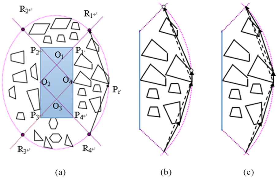
Process of generating rbCH: (a) find the first vertex, (b) construct directed edges and find the V_furthest, and (c) renewal of directed edge is finished.

S ₁ = {H₁, H₂,…, H_i,…, H_n} = {P₁, P₂,…, P_n₁}, where H_i is the set of vertexes of the ith stock part constructed by PiCH. H is the set of vertexes in rbCH having q numbers of vertexes. $H = {H'_{1}, H'_{2}, \dots, H'_{i}, \dots, H'_{n}} = {O_{1}, O_{2}, \dots, O_{q}}$ , where $H'_{i}$ is the set of vertexes of the ith stock part in set H_i:

Step 1: Point P_r is the farthest from point O_2. Points R₁, P₁, P₄, R₄, and P_r (counterclockwise (CCW)) are initial rbCH defined as set of H. Delete the points in the polygon region R₁P₁P₄R₄P_r from the set of S₁. If S₁ is null, turn to step 5, else turn to step 2;

Step 2: Connecting the vertexes in set H constructs directed edges. Search the outer points of the directed edges in set S₁ and delete the inner points. Find the vertexes right to each directed edge and compare the distance of these vertexes away from the edge. The farthest is V_furthest;

Step 3: Add V_furthest into the set H, and update the border of the polygon of H. Delete the inner points of new polygon of H from set S₁;

Step 4: If S₁ is null, turn to step 5, else turn to step 2;

Step 5: Return to the vertexes of rbCH, end.

Convex decomposition of concave polygon

If there are some concave polygons in the packing of irregular polygon items, most of the handling method is complementary convex or convex decomposition of concave polygon techniques at present. Complementary convex as shown in Figure 13(b) substituting nonconvex polygon as shown in Figure 13(a) would reduce the utilization rate of material. Convex decomposition of concave polygon adds some subdivision lines to make the concave polygon into several convex polygons to participate in the layout process.

Figure 13.

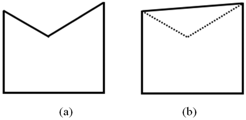
Nonconvex polygon and its complementary convex: (a) concave polygon and (b) complementary convex.

Conventional subdivision technologies deal with all vertexes and do an optimal subdivision to obtain a good form as much as possible. In this article, the form requirement of convex polygon is not high. So, it uses only one concave point and other points-of-visibility to subdivide a concave polygon into several convex polygons and simple concave polygons quickly and then subdividing could continue until no concave.

Definition: point-of-visibility

For any one vertex, if the line segments that attach this vertex and other vertexes are all within the polygon or above the edges, then these are called points-of-visibility. P₄ and P₉ are the points-of-visibility of P₁ (Figure 14(a)). Judgment method is as follows: Suppose the present concave point as P_i, P_n as the last point in CCW, and P_i_+x is under judgment. Line F(x, y) connects P_i and P_i_+x. If the points between P_i and P_i_+x−1 are all at the right hand of F(x, y), and points between the P_i_+x+1 and P_n are all at the left, P_i_+x would be the point-of-visibility. Otherwise, it would be point-of-invisibility.

Figure 14.

Convex decomposition at different concave polygon points: (a) P₁, (b) P₅, (c) P₇, and P₈.

The principle of convex decomposition is as follows: Connecting a concave point and all vertexes in CCW would obtain some triangles, which are convex polygons. But if there are some points-of-invisibility, the related subdivision lines are not improper, so concave polygon still exists. Continue to subdivide this concave polygon according to this principle of subdivision and obtain the final result. Adjacent triangles can also merge into a new convex polygon.

The algorithm for different concave point complexities is different, as shown in Figure 14. P₁ has two points-of-invisibility, P₅ has four points-of-invisibility, P₇ has three points-of-invisibility, and P₈ has four points-of-invisibility. Selecting P₁ will, therefore, reduce the operation complexity.

Algorithm is shown as follows:

Step 1: Search all the concave points from the first vertex of the polygon and record it;

Step 2: Judge the points are visibility or not for each concave point, record the string of vertexes in CCW, and tag it with visibility and invisibility. Select the concave point P that has less points-of-invisibility to be the start of subdivision lines;

Step 3: Connect P and other adjacent vertexes in sequence. If the current vertex is point-of-invisibility, turn to step 4, else turn to step 5;

Step 4: Delete the line of this vertex and P and connect P and the next vertex. If the current point is point-of-invisibility, step 4 is repeated until the current point is point-of-visibility. Add the current subdivision line. But this polygon subdivided just now is concave polygon, so continue further decomposition, else turn to step 1;

Step 5: This polygon subdivided just now is a triangle and is a convex polygon;

Step 6: Connect the next vertex. If this vertex is point-of-invisibility, turn to step 4, else judge whether the polygon merges this polygon subdivided just now and the prior convex polygon is also a convex polygon or not. If yes, delete the prior subdivision line. If not, add the current subdivision line and then turn to step 6, until the last nonadjacent.

Force analysis

In order to simulate the physical movements of a set of items wrapped by a rubber band, a plural vector expression approach is adopted. Here, we just compute the direction of the force vector. The size is given by adaptive module as shown in section “Rubber band force and time step based on adaptive function.” As mentioned (section “rbCH”) earlier, $H = {H'_{1}, H'_{2}, \dots, H'_{i}, \dots, H'_{n}} = {O_{1}, O_{2}, \dots, O_{q}}$ is the set of rbCH. The tension of rubber band is a vector invariable in packing course as mentioned above. This vector is normalized to a unit vector, whose direction is from current vertex directing to next vertex. The resultant vector acting on each item is calculated by taking a vector sum of all those vectors acting on that item. Suppose the ith item have x₂ vertexes from x₁th vertex on rbCH. Figure 15 and formula (12) show how to composite the resultant of F about one item, where $\vec{F_{i 1}}$ and $\vec{F_{i 2}}$ computed by formulas (13)–(16) are unit vector forces along the vector side of rbCH

\vec{F_{i}} = \vec{F_{i 1}} + \vec{F_{i 2}}

(12)

\vec{f_{i 1}} = P_{x_{1}} P_{x_{1} - 1} = (X_{P_{x_{1}}} - X_{P_{x_{1} - 1}}) + (Y_{P_{x_{1}}} - Y_{P_{x_{1} - 1}}) i

(13)

\vec{f_{i 2}} = P_{x_{1} + x_{2} - 1} P_{x_{1} + x_{2}} = (X_{P_{x_{1} + x_{2} - 1}} - X_{P_{x_{1} + x_{2}}}) + (Y_{P_{x_{1} + x_{2} - 1}} - Y_{P_{x_{1} + x_{2}}}) i

(14)

\vec{F_{i 1}} = \frac{\vec{f_{i 1}}}{| \vec{f_{i 1}} |}

(15)

\vec{F_{i 2}} = \frac{\vec{f_{i 2}}}{| \vec{f_{i 2}} |}

(16)

Figure 15.

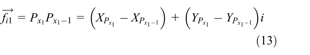
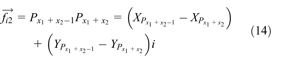
Force analysis.

Experimental results

In this section, NestRB system is tested based on the nesting problem of sheet metal cutting. The proposed method is here evaluated using the problems created by us and some benchmark problems that are available from the Euro Special Interest Group on Cutting and Packing (ESICUP) website.²⁵ Each problem is run at 20 times and then the best result of PD is picked as shown in sections “Some problems created by us,”“One set of benchmark problems,” and “Another set of benchmark problems,” which is tested with the following three advantages:

Each step of the iterative result could be seen in the process of packing movement;

The execution time is short;

Good solution.

Some problems created by us

The NestRB system is developed by Visual C++. We conducted our system on personal computer with Windows 7 operation system, with a 3-GHz Intel Pentium4 630 processor and with 2-GB DDR3 1333 RAM. The packing process of the NestRB system would be shown by a problem created by us like jigsaw puzzle whose solution is good, 91.4%. We measured the quality of solutions utilizing the PD (equation (2)) of the packing. The three figures intercepted from packing process show the different statuses in movement, which is a perceptual intuition. The tolerance zone is set as the gap of cutting tool machining between the items. Figure 16(a) shows the packing items prepacked into the four regions of all around the sheet according to the area and the length side, and then rbCHs are generated. Figure 16(b) shows one step of the packed process about the shrinking of the rubber band. Figure 16(c) shows the final packing status after the rubber band packing process. The proposed method packed items in short times of 20.25 s with perceptual intuition which shows each step of the iterative results. The other jigsaw puzzle is a problem that makes a hexagon split in six hexagons and then the rubber band makes them together to gain a good PD, 97.2%. Figure 17(b) and (c) shows regular layout problems, 72 hexagons and 95 circles, and also good solutions in execution time and PD.Table 1 lists the results of the problems created by us.

Figure 16.

One jigsaw puzzle: (a) first illustration showing one process of packing, (b) second illustration showing one process of packing, and (c) packing result.

Figure 17.

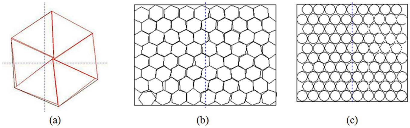
Some problems created by us: (a) the other jigsaw puzzle, (b) 72 hexagons, and (c) 95 circles.

Table 1.

Results of the problems created by us.

Problem created by us	Sheet width	Item types	Items	Best solution (average)	Time (s)	Item size
One jigsaw puzzle	40	32	32	93.7% (89.5%)	20.25	Appendix 1
Other jigsaw puzzle	–	1	6	97.2% (96.8%)	8.53	Length = 10
72 Hexagons	400	1	72	87.2% (85.6%)	15.32	Length = 22
95 Circles	120	1	95	84.4% (83.9%)	14.46	Diameter = 20

One set of benchmark problems

We compare our proposed method with some well-known benchmark problems. Of the benchmark problems under consideration, five were produced by Hopper⁹ including convex and nonconvex polygonal shapes. Their size varies from 15 to 75 packing items. The other three benchmark problems also have been artificially created including convex and nonconvex polygonal shapes. We measure the quality of solutions utilizing the PD (equation (2)) of the packing when the width is fixed. The results are listed according to the presented references in Table 2. The overall quality of the layouts produced by NestRB system is outstanding in both PD and execution times. The problems of Poly1a, Poly2a, Poly3a, Poly4a, and Poly5a created by Hopper⁹ are solved with low PD (below 70%), whereas Burke et al.¹⁴ and Liu and Ye¹⁹ solved them with high PD (over 70%). But our approach could lead to solutions of better quality to reach their value or beyond them. Besides good PD, execution time is very short. The more the packing items, the longer the execution time with our approach. Poly5a problem has 75 packing items, solving it with our approach only consuming 287.3 s, 1/17th of the times of Burke et al.¹⁴ So, the execution time has absolute advantage.

Table 2.

Results of the literature benchmark problems and our approach.

Problem	Reference	Width	Item types	Items	Best solution (and average solution)	Admissible orientations (°)	Time (s)
Poly1a	Hopper⁹	40	15	15	59.6%	0	1380
	SigmaNest⁹				59.9%	0	–
	NestLib⁹				69.7%	0	–
	Burke et al.¹⁴				73.2%	0	360
	Stoyan et al.²³				77.6%	Free rotation	150
	Our approach				73.2% (71.8%)	Free rotation	27.59
Poly2a	Hopper⁹	40	15	30	61.4%	0	2940
	SigmaNest⁹				67.5%	0	–
	NestLib⁹				68.1%	0	–
	Burke et al.¹⁴				72.8%	0	1240
	Stoyan et al.²³				79.7%	Free rotation	280
	Our approach				76.3% (75.6%)	Free rotation	61.23
Poly3a	Hopper⁹	40	15	45	60.4%	0	4500
	SigmaNest⁹				68.3%	0	–
	NestLib⁹				76.1%	0	–
	Burke et al.¹⁴				73.8%	0	2010
	Stoyan et al.²³				79.2%	Free rotation	390
	Our approach				77.3% (74.9%)	Free rotation	149.66
Poly4a	Hopper⁹	40	15	60	60.2%	0	7020
	SigmaNest⁹				69.1%	0	–
	NestLib⁹				72.1%	0	–
	Burke et al.¹⁴				74.6%	0	2430
	Stoyan et al.²³				78.7%	Free rotation	410
	Our approach				79.6% (78.9%)	Free rotation	210.74
Poly5a	Hopper⁹	40	15	70	59.3%	0	8880
	SigmaNest⁹				69.4%	0	–
	NestLib⁹				71.6%	0	–
	Burke et al.¹⁴				73.9%	0	5040
	Stoyan et al.²³				80.3%	Free rotation	867
	Our approach				77.5% (72.8%)	Free rotation	287.32
Blaz1	Martins and Tsuzuki¹²	15	7	28	72.89%	0, 180	1066.02
	Valle et al.²⁶				91.8%	0, 180	59.85
	Gomes and Oliveira¹⁰				81.41%	0, 180	2136
	Liu and Ye¹⁹				76.21%	0, 180	18
	Our approach				74.5% (72.4%)	Free rotation	56.86
Jakobs1	Martins et al.¹²	40	25	25	75.3%	0, 90, 180, 270	67.79
	Valle et al.²⁶				98.7%	0, 90, 180, 270	109.09
	Gomes and Oliveira¹⁰				75.79%	0, 90, 180, 270	332
	Liu and Ye¹⁹				75.38%	0, 90, 180, 270	59
	Stoyan et al.²³				82.9%	Free rotation	495
	Elkeran²⁷				89.10%	0, 90, 180, 270	600
	Our approach				73.7% (72.5%)	Free rotation	48.46
Jakobs2	Martins et al.¹²	70	25	25	68.4%	0, 90, 180, 270	619.51
	Valle et al.²⁶				98.5%	0, 90, 180, 270	119.88
	Gomes and Oliveira¹⁰				74.66%	0, 90, 180, 270	454
	Liu and Ye¹⁹				72.11%	0, 90, 180, 270	183
	Elkeran²⁷				87.73%	0, 90, 180, 270	600
	Our approach				79.4% (75.1%)	Free rotation	53.67

The problems of Blaz1, Jakobs1, and Jakobs2 have good solutions, for example, Valle et al.²⁶ give PD with 98.7%, 91.8%, and 98.7%, respectively. So does Elkeran²⁷ on the problems of Jakobs1 and Jakobs2. Our approach limited by the initial layout could not reach that performance, but we have advantages in the execution time with 56.86, 48.46, and 53.67 s, respectively. Besides, our system could be intuitive to observe dynamic layout process.

Comparing with Stoyan et al.’s²³ approach which also allows free rotation, our approach is superior with respect to execution time but failure with respect to PD. Finally, the best layout obtained in our computational tests for each problem instance is presented in Figure 18.

Figure 18.

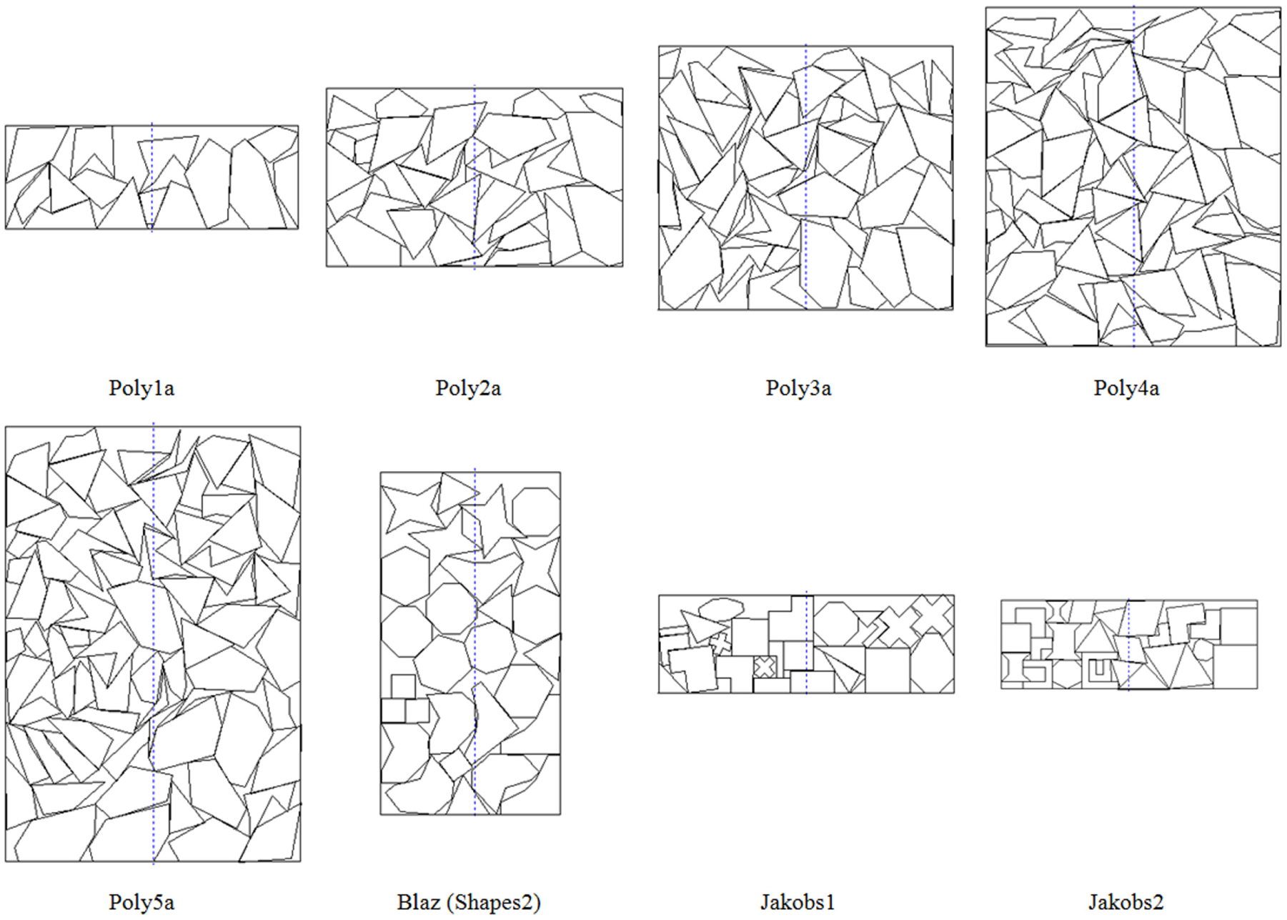
Our solution for some benchmark problems.

Another set of benchmark problems

We compared the proposed method with benchmark problems. Table 3 summarizes the performance of this work and other methods from the literature, when they are applied to the cutting problem about shirts, trousers, Dagli, Marques, and Albano. Our system achieves better packing densities than much solution methods, for example, merit in Hopper,⁹ SigmaNest,⁹ and NestLib⁹ for shirt problem. When our system is not outstanding in packing densities, then we are faster, for example, merit in Burke et al.,¹⁴ Gomes,¹⁰ Nielsen and Odgaard,¹⁶ and Oliveira et al.⁸ for shirt problem. Our approach solves this set of garment benchmark problems that spent more time than the problem mentioned in the previous section. Besides, our system could be intuitive to observe dynamic layout process. Finally, the best layout obtained in our computational tests for each problem instance is presented in Figure 19.

Table 3.

Results of the literature garment benchmark problems and our approach.

Problem	Reference	Width	Item types	Items	Admissible orientations (°)	Best solution (and average solution)	Time (s)
Shirts	Hopper⁹	40	8	99	0, 180	79.6%	–
	SigmaNest⁹				0, 180	72.2%	–
	NestLib⁹				0, 180	78.1%	–
	Burke et al.¹⁴				0, 180	84.6%	4990
	Gomes and Oliveira¹⁰				0, 180	86.79%	10391
	Nielsen and Odgaard¹⁶				0, 180	86.5%	3600
	Oliveira et al.⁸				0, 180	81.3%	210.5
	Elkeran²⁷				0, 180	88.96%	1200
	Our approach				Free rotation	81.8% (74.6%)	340.89
Trousers	Hopper⁹	79	17	64	0, 180	76.7%	–
	SigmaNest⁹				0, 180	79.1%	–
	NestLib⁹				0, 180	76.8%	–
	Burke et al.¹⁴				0, 180	88.5%	7890
	Gomes¹²				0, 180	89.96%	8588
	Nielsen and Odgaard¹⁶				0, 180	89.8%	3600
	Oliveira et al.⁸				0, 180	82.8%	187.7
	Elkeran²⁷				0, 180	91.00%	1200
	Dalalah et al.²⁸				0, 180	82.97%	520
	Our approach				Free rotation	86.4% (82.8%)	265.48
Dagli	Hopper⁹	60	10	30	0, 180	72.5%	–
	SigmaNest⁹				0, 180	75.6%	–
	NestLib⁹				0, 180	77.3%	–
	Burke et al.¹⁴				0, 180	83.7%	2040
	Gomes and Oliveira¹⁰				0, 180	87.15%	5110
	Liu and Ye¹⁹				0, 180	83.48%	219
	Elkeran²⁷				0, 180	89.51%	1200
	Our approach				Free rotation	85.6% (84.2%)	132.58
Marques	Gomes and Oliveira¹⁰	104	8	24	0, 90, 180, 270	88.14%	7507
	Liu and Ye¹⁹				0, 90, 180, 270	84.05%	369
	Elkeran²⁷				0, 90, 180, 270	90.59%	1200
	Our approach				Free rotation	81.4%	118.12
Albano	Gomes and Oliveira¹⁰	4900	8	24	0, 180	87.43%	2257
	Elkeran²⁷				0, 180	89.58%	2100
	Our approach				Free rotation	86.7% (84.5%)	124.39

Figure 19.

Our solution for some garment benchmark problems: (a) shirts, trousers, and Dagli and (b) Marques and Albano.

Conclusion

Packing problems exist almost everywhere in real-world situation. Since it can be noted that irregular item packing problems are more complex than regular ones, the focus of this article is on the irregular object packing problems. In this study, a novel rubber band analogy algorithm packing approach based on the physical method is proposed to establish an effective methodology for achieving an efficient allocation of irregular items in a stock sheet of fixed width without overlap. In particular, the presented algorithm performs better than the approaches from other in perceptual intuition, while producing solutions of better quality than some benchmark problems.

Although the main advantage of our NestRB system is its ability to translate, slide, and rotate the items into a compact layout obtaining a good solution in an acceptable time, the initial position of the packing items is at random, and how to choose the initial position for the items is still not clear. This could be an interesting research question for future studies.

Footnotes

Appendix 1

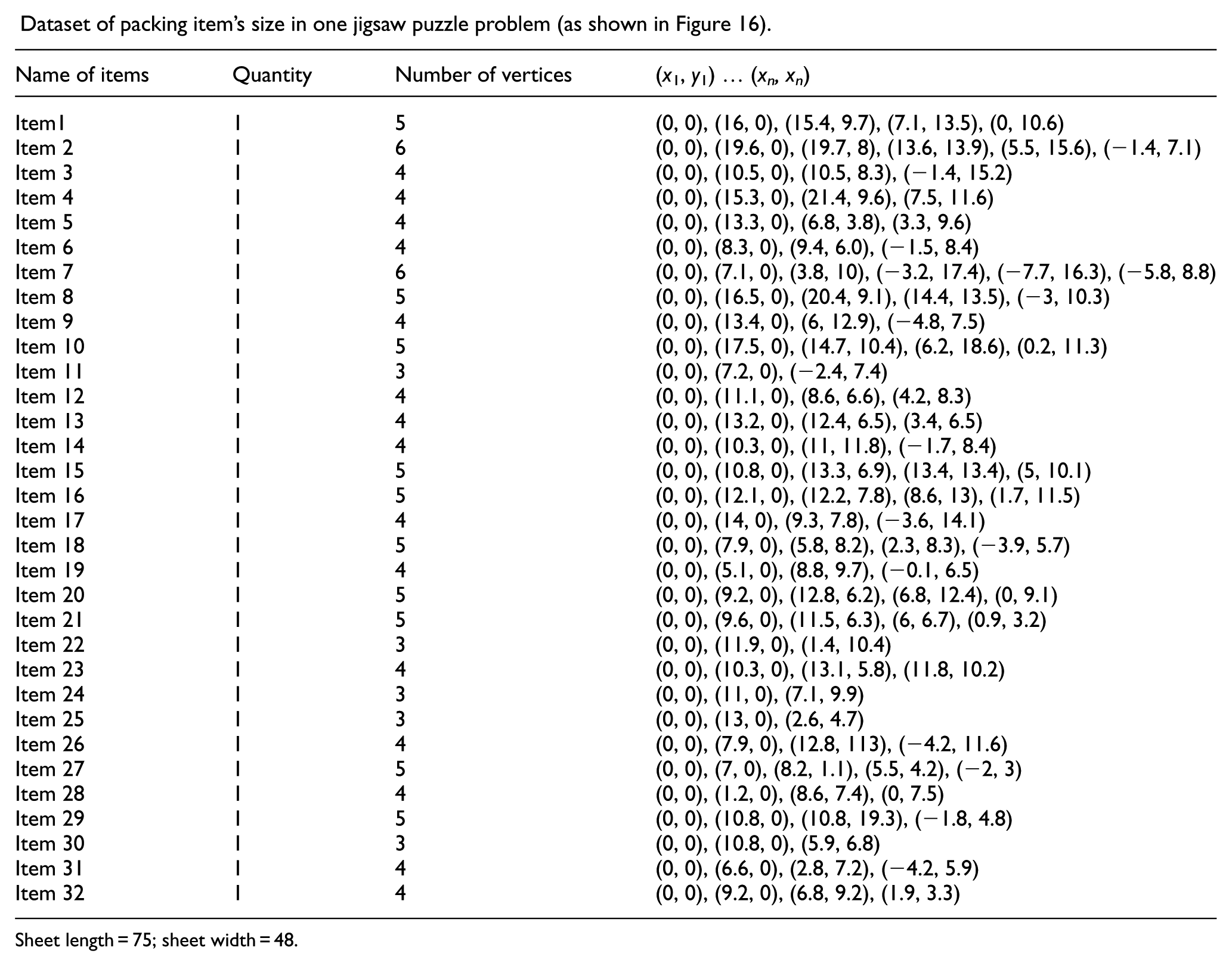
Dataset of packing item’s size in one jigsaw puzzle problem (as shown in Figure 16).

Name of items	Quantity	Number of vertices	(x₁, y₁) … (x_n, x_n)
Item1	1	5	(0, 0), (16, 0), (15.4, 9.7), (7.1, 13.5), (0, 10.6)
Item 2	1	6	(0, 0), (19.6, 0), (19.7, 8), (13.6, 13.9), (5.5, 15.6), (−1.4, 7.1)
Item 3	1	4	(0, 0), (10.5, 0), (10.5, 8.3), (−1.4, 15.2)
Item 4	1	4	(0, 0), (15.3, 0), (21.4, 9.6), (7.5, 11.6)
Item 5	1	4	(0, 0), (13.3, 0), (6.8, 3.8), (3.3, 9.6)
Item 6	1	4	(0, 0), (8.3, 0), (9.4, 6.0), (−1.5, 8.4)
Item 7	1	6	(0, 0), (7.1, 0), (3.8, 10), (−3.2, 17.4), (−7.7, 16.3), (−5.8, 8.8)
Item 8	1	5	(0, 0), (16.5, 0), (20.4, 9.1), (14.4, 13.5), (−3, 10.3)
Item 9	1	4	(0, 0), (13.4, 0), (6, 12.9), (−4.8, 7.5)
Item 10	1	5	(0, 0), (17.5, 0), (14.7, 10.4), (6.2, 18.6), (0.2, 11.3)
Item 11	1	3	(0, 0), (7.2, 0), (−2.4, 7.4)
Item 12	1	4	(0, 0), (11.1, 0), (8.6, 6.6), (4.2, 8.3)
Item 13	1	4	(0, 0), (13.2, 0), (12.4, 6.5), (3.4, 6.5)
Item 14	1	4	(0, 0), (10.3, 0), (11, 11.8), (−1.7, 8.4)
Item 15	1	5	(0, 0), (10.8, 0), (13.3, 6.9), (13.4, 13.4), (5, 10.1)
Item 16	1	5	(0, 0), (12.1, 0), (12.2, 7.8), (8.6, 13), (1.7, 11.5)
Item 17	1	4	(0, 0), (14, 0), (9.3, 7.8), (−3.6, 14.1)
Item 18	1	5	(0, 0), (7.9, 0), (5.8, 8.2), (2.3, 8.3), (−3.9, 5.7)
Item 19	1	4	(0, 0), (5.1, 0), (8.8, 9.7), (−0.1, 6.5)
Item 20	1	5	(0, 0), (9.2, 0), (12.8, 6.2), (6.8, 12.4), (0, 9.1)
Item 21	1	5	(0, 0), (9.6, 0), (11.5, 6.3), (6, 6.7), (0.9, 3.2)
Item 22	1	3	(0, 0), (11.9, 0), (1.4, 10.4)
Item 23	1	4	(0, 0), (10.3, 0), (13.1, 5.8), (11.8, 10.2)
Item 24	1	3	(0, 0), (11, 0), (7.1, 9.9)
Item 25	1	3	(0, 0), (13, 0), (2.6, 4.7)
Item 26	1	4	(0, 0), (7.9, 0), (12.8, 113), (−4.2, 11.6)
Item 27	1	5	(0, 0), (7, 0), (8.2, 1.1), (5.5, 4.2), (−2, 3)
Item 28	1	4	(0, 0), (1.2, 0), (8.6, 7.4), (0, 7.5)
Item 29	1	5	(0, 0), (10.8, 0), (10.8, 19.3), (−1.8, 4.8)
Item 30	1	3	(0, 0), (10.8, 0), (5.9, 6.8)
Item 31	1	4	(0, 0), (6.6, 0), (2.8, 7.2), (−4.2, 5.9)
Item 32	1	4	(0, 0), (9.2, 0), (6.8, 9.2), (1.9, 3.3)

Sheet length = 75; sheet width = 48.

Academic Editor: Neal Y Lii

Declaration of conflicting interests

The author(s) declared no potential conflicts of interest with respect to the research, authorship, and/or publication of this article.

Funding

The author(s) disclosed receipt of the following financial support for the research, authorship, and/or publication of this article: This work was financially supported by Natural Science Foundation of China (51265002) and Key Laboratory of Manufacturing System and Advance Manufacturing Technology of GuangXi Province (12-071-11S04).

References

Hopper

Turton

BCH

. A review of the application of meta-heuristic algorithms to 2D strip packing problems. Artif Intell Rev 2001; 16: 257–300.

Bennell

Oliveira

JF.

A tutorial in irregular shape packing problems. J Oper Res Soc 2009; 60: 93–105.

Paull

AE.

Linear programming: a key to optimum newsprint product. Pulp Paper Mag Can 1956; 5: 145–150.

Huang

Shi

A better nesting method for sheet metal CAD. J Comput Aided Des Comput Graph 2000; 12: 380–383.

Xue

Sun

Rectangle packing optimization utilizing hybrid genetic algorithms. Comput Eng Des 2007; 28: 5457–5460.

Chaudhuri

Samal

A simple method for fitting of bounding rectangle to closed regions. Pattern Recogn 2007; 40: 1981–1989.

Dagli

. Cutting stock problem: combined use of heuristics and optimization methods. In: Proceedings 9th international conference on production research, Cincinnati, US, August 1987, pp.843–849.

Oliveira

Gomes

Ferreira

JS.

TOPOS—a new constructive algorithm for nesting problems. OR Spektrum 2000; 22: 263–284.

Hopper

Two-dimensional packing utilizing evolutionary algorithms and other meta-heuristic methods. PhD Thesis, University of Wales, Cardiff, 2000.

10.

Gomes

Oliveira

JF.

Solving irregular strip packing problems by hybridizing simulated annealing and linear programming. Eur J Oper Res 2006; 171: 811–829.

11.

Hifi

M’Hallah

A hybrid algorithm for the two-dimensional layout problem: the cases of regular and irregular shapes. Int Trans Oper Res 2003; 10: 195–216.

12.

Martins

Tsuzuki

MSG

. Simulated annealing applied to the irregular rotational placement of shapes over containers with fixed dimensions. Expert Syst Appl 2010; 37: 1955–1972.

13.

Dowsland

Vaid

Dowsland

WB.

An algorithm for polygon placement using a bottom-left strategy. Eur J Oper Res 2002; 141: 371–381.

14.

Burke

Hellier

Kendall

. A new bottom left-fill heuristic algorithm for the two-dimensional irregular packing problem. Oper Res 2006; 54: 587–601.

15.

Weng

Kuo

HC.

Irregular stock cutting system based on AutoCAD. Adv Eng Softw 2011; 42: 634–643.

16.

Nielsen

Odgaard

Fast neighborhood search for the nesting problem. Technical report, University of Copenhagen, Copenhagen, 2003.

17.

Dowsland

WB.

Solution approaches to irregular nesting problems. Eur J Oper Res 1995; 84: 506–521.

18.

Liu

YJ.

Algorithm for 2-D irregular-shaped nesting problem based on the NFP algorithm and lowest-gravity-center principle. J Zhejiang Univ: Sc A 2006; 7: 570–576.

19.

Liu

JW.

Heuristic algorithm based on the principle of minimum total potential energy (HAPE): a new algorithm for nesting problems. J Zhejiang Univ: Sc A (Appl Phys & Eng) 2011; 12: 860–872.

20.

Milenkovic

Compaction and separation algorithms for nonconvex polygons and their applications. Eur J Oper Res 1995; 84: 539–561.

21.

Fadel

Sinha

Packing optimization using a rubber band analogy. In: Proceedings of ASME design engineering technical conference, Pittsburgh, PA, 9–12 September 2001, pp.409–415. New York: ASME.

22.

Dong

Fadel

Blouin

VY.

Packing optimization by enhanced rubber band analogy. In: Proceedings of ASME design engineering technical conference, Long Beach, CA, 24–28 September 2005, pp.681–689. New York: ASME.

23.

Stoyan

Zlotnik

Chugay

AM.

Solving an optimization packing problem of circles and non-convex polygons with rotations into a multiply connected region. J Oper Res Soc 2012; 63: 379–391.

24.

Bouganis

Shanahan

A vision-based intelligent system for packing 2-D irregular shapes. IEEE T Autom Sci Eng 2007; 4: 382–394.

25.

Euro Special Interest Group on Cutting and Packing (ESICUP), http://www.apdio.pt/esicup

26.

Valle

AMD

Queiroz

TAD

Miyazawa

. Heuristics for two-dimensional knapsack and cutting stock problems with items of irregular shape. Expert Syst Appl 2012; 39: 12589–12598.

27.

Elkeran

A new approach for sheet nesting problem using guided cuckoo search and pair wise clustering. Eur J Oper Res 2013; 231: 757–769.

28.

Dalalah

Khrais

Bataineh

Waste minimization in irregular stock cutting. J Manuf Syst 2014; 2014: 27–40.

Visual nesting system for irregular cutting-stock problem based on rubber band packing algorithm

Abstract

Keywords

Introduction

Related works

New approach for the nesting system

Definition

RBPA

Improved RBPA for NestRB system

Some key problems of the NestRB system

Rubber band force and time step based on adaptive function

Packing item geometry identification and data structure

rbCH

Convex decomposition of concave polygon

Definition: point-of-visibility

Force analysis

Experimental results

Some problems created by us

One set of benchmark problems

Another set of benchmark problems

Conclusion

Footnotes

Appendix 1

Declaration of conflicting interests

Funding

References