Sage Journals: Discover world-class research

Abstract

Interaction of current with circular cylinders near a rigid bed is significant in the design of offshore structures, such as pipelines. Pipelines are buried to the seabed to be protected from damages caused by hydrodynamic forces or human activities. The pipeline laid on movable bed can be buried due to local scouring. A vertical plate on pipeline, called spoiler, has been developed to increase the rate and extend of scouring. In this study, the two-dimensional turbulent flow around a smooth pipeline with a spoiler was investigated at Re_D = 9500 near the bed. The governing equations for the current problem were solved using ANSYS^® 11.0-Flotran program package based on finite element method. The performance of the standard k–ε, standard k–ω, and shear stress transport turbulence models were examined on five computational meshes with different densities. The results obtained were compared with the published experimental measurements in literature. Present results showed that the attachment of a spoiler caused a large separation area in both upstream and downstream of the pipeline. The attachment of spoiler on top of the pipe increased the drag and decreased the lift force on pipe. Moreover, the spoiler causes non-zero downward lift. It is concluded that the k–ω turbulence model on the finest mesh is found relatively better in simulation of the flow field.

Keywords

Spoiler pipeline separation area turbulence flow field

Introduction

The interaction between the fluid flow and the bluff bodies near to erodible bed is important in engineering applications, that is, submarine pipelines. It is crucial for the engineering designs to define the flow field around the body and the hydrodynamic forces. The flow around a circular cylinder without a spoiler (wall affect, vortex shedding, vortex suppression, flow area, etc.) has been investigated experimentally^1–7 and theoretically^8–12 by many researchers in the past.

Submarine pipelines laid on the seabed are exposed to the current causing local scour on the erodible bed below the pipeline. Consequently, free spans can develop or be formed as gaps between the bed and pipeline. The onset and mechanism of scour have been studied by Mao,¹³ Chiew,¹⁴ Sumer and Fredsoe,¹⁵ Kolmp et al.,¹⁶ Liang and Cheng,¹⁰ Dey and Singh,¹⁷ Zang et al.,¹⁸ Cheng et al.,¹⁹ Gao and Luo,²⁰ and Arya and Shingan.²¹

The pipelines are often buried or trenched, to be protected from hydrodynamic forces or from human activities such as fishing gear. The trenching or burial of pipelines underneath the seabed, by all means, increases the cost of a pipeline projects. Past studies^10,13–19 showed that pipelines can be buried naturally under convenient situations. A vertical plate called “spoiler” attached on top of the pipeline has been developed to accelerate the self-burial of the pipeline and to increase extend of scour hole. It is reported that^22–24 attaching a spoiler on a pipeline not only increases the amount and intensity of scours but also leads to 10 times faster self-burial compared to a pipeline without spoiler.

The theoretical and experimental studies^25–27 reported that the main factors causing an increase in the amount of the scours are blockages effect and the increase in the rate of the flow between the bed and pipeline due to the inserted spoiler. It is stated that the spoiler on a pipeline increases the width of the wake and delay or suppressed the appearance of regular vortex shedding by disrupting the interaction between the vortex pairs, and besides, it is necessary to take into consideration the mentioned points related to designing a pipeline with a spoiler since it influences the hydrodynamic force distributions on a pipeline. Moreover, it is known that attaching a spoiler to a pipe increases the dimensions of upstream and downstream separation areas. Therefore, more energetic vorticity regions are formed due to the increase in the separation areas resulting with speeding up seepage transpiring on the seabed and, thus, increasing the intensity and amount of scours.^13,28

It is observed that although pipelines with spoiler are practiced in tens of projects, the data published in literature regarding the effect of a spoiler mounted on a pipeline are still not sufficient; thus, a study on this subject has a great importance in terms of industrial application. In this study, the analyses of flow field around a circular cylinder with spoiler are investigated numerically, with gap ratio G/D (G: gap between the bed and the pipe; D: diameter of the pipe) = 0.0, 0.1, 0.2, and 0.3 at Re_D(= u₀D/ν) = 9500. The numerical velocity fields, drag, and lift coefficients for a pipeline with spoiler were determined using the ANSYS^® 11-CFD program package, and numerical results are compared with experimental measurements of Zdravkovich,² Cheng and Chew,²⁷Öner,²⁸Öner and Kırkgöz,²⁹Öner et al.,⁷ and Choi and Lee.³ Moreover, the influence of mesh density on computational results using standard k–ε, standard k–ω, and shear stress transport (SST) turbulence closure models is evaluated.

Governing equations

In this study, the flow field around a pipeline laid on a plane is modeled using the incompressible two-dimensional (2D) Reynolds-averaged continuity and Navier–Stokes equations

\frac{\partial u_{i}}{\partial x_{i}} = 0

(1)

ρ u_{j} \frac{\partial u_{i}}{\partial x_{j}} + ρ \frac{\partial u_{i}}{\partial t} = ρ K_{i} - \frac{\partial p}{\partial x_{i}} + μ \frac{\partial^{2} u_{i}}{\partial x_{j} \partial x_{j}} + \frac{\partial}{\partial x_{j}} (- ρ \bar{{u'}_{i} {u'}_{j}})

(2)

In equations (1) and (2), $u_{i}$ represent the velocity components in x_i direction; $ρ$ is the density of fluid; K is the body force due to gravity; p is the pressure; $μ$ is the dynamic viscosity; $(- ρ \bar{{u'}_{i} {u'}_{j}}) (= τ_{ij})$ is the turbulent (Reynolds) stress, $u'_{i}$ and $u'_{j}$ are the horizontal and vertical velocity fluctuations, respectively. The turbulent stresses in equation (2) can be obtained from the constitutive equation defined as in the following

τ' = - ρ \bar{{u'}_{i} {u'}_{j}} = η (\frac{\partial u_{i}}{\partial x_{j}} + \frac{\partial u_{j}}{\partial x_{i}}) - \frac{2}{3} ρ k δ_{ij}

(3)

where k is the turbulence kinetic energy, δ_ij is the Kronecker delta, and η is the turbulent or eddy viscosity coefficient. Various turbulence closure models in computational fluid dynamics (CFD) simulations have been used to determine the turbulent viscosity, η, in equation (3).^30–34 In the present numerical simulation, standard k–ε,³²k–ω,³³ and SST³⁴ turbulence closure models were employed.

Standard k–ε turbulence closure model is a well-known two-equation turbulence model which expresses the turbulence viscosity in terms of kinetic energy, k, and its dissipation rate, ε. Another two-equation turbulence closure model is the k–ω model which is less commonly used compared to the k–ε model. k–ω turbulence closure model was reported to have the advantages near the walls to predict the turbulence length scale (ℓ ~ k^1/2/ω) accurately in the presence of adverse pressure gradient boundary layer flow.³³ To combine the advantages of k–ε and k–ω models, Menter³⁴ presented the SST turbulence closure model that uses a blending function, F₁, which ensures smooth transition between the k–ω model near the wall regions and k–ε away from the wall. Thus, SST model coefficients reduce to the k–ω and k–ε model coefficients in their respective regions. The reader is referred to Launder and Spalding,³² Menter,³⁴ Wilcox,^31,33 and Akoz et al.³⁵ for details.

Liang and Cheng¹⁰ investigated the effect of turbulence closure models on the simulation of flow around a pipeline and concluded that k–ω model with no-slip boundary condition on the cylinder surface gave better results compared to the wall function boundary conditions in predictions of shedding of the vortices. Kırkgöz et al.³⁶ investigated 2D flow around a smooth cylinder near a rigid bed with G/D = 0.3 and Re_D = 9500. Kırkgöz et al.³⁶ compared the k–ε, k–ω, and SST turbulence closure models on different mesh densities. Kırkgöz et al.³⁶ concluded that in the simulation of the flow field around the cylinder, k–ω and SST turbulence closure models for the best mesh gave almost equally best predicted computational results. Aköz and Kırkgöz³⁷ studied numerically and experimentally the flow around a horizontal wall-mounted circular cylinder and compared the effect of turbulence closure models on results. They indicated that numerical modeling using k–ω and SST turbulence closure models is reasonably successful, and the computational results predicted by k–ω and SST are similar to each other. Kazeminezhad et al.³⁸ investigated the force components and vortex shedding frequency of a pipe exposed to steady current. Kazeminezhad et al.³⁸ numerically solved the flow area around a pipe using the Reynolds-averaged Navier–Stokes equations with the k–ε turbulence closure model. They indicated that the model well predicted the velocity profile around the pipe, whereas slightly over-predicts the mean force coefficients and Strouhal number.

Numerical method and solution domain

Numerical method

The numerical solution of the Reynolds-averaged continuity and Navier–Stokes equations (equations (1) and (2)) are obtained using ANSYS^®/FLOTRAN CFD package based on finite element methods. In the finite element discretization, the conservation forms of equations (1) and (2) were used. There, for a transferable fluid property, ϕ is defined per unit mass in a unit control volume as

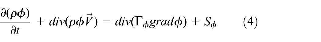
\frac{\partial (ρ ϕ)}{\partial t} + div (ρ ϕ \vec{V}) = div (Γ_{ϕ} grad ϕ) + S_{ϕ}

(4)

In equation (4), $\vec{V}$ , $Γ_{ϕ}$ , and $S_{ϕ}$ are the velocity vector, generalized diffusion coefficient, and generalized source term, respectively. The value of the fluid property “ϕ” is 1 for the conservation of mass, and it is $\vec{V}$ for the conservation of momentum.

Solution domain and boundary conditions

In this study, a rectangle with 2.0 m length and 0.32 m width was considered as the solution domain that was identical with experimental conditions of Öner²⁸ in the channel. As seen in Figure 1, a circular cylinder with a diameter of D = 50 mm and a height of 10 mm spoiler was mounted on the channel bed, center of the cylinder is located at x = 1500 mm (30D) in the domain from the left and 500 mm (10D) from the right. Long distance of calculation domain was considered in front of the cylinder to compute the deformation of the flow around cylinder accurately.³⁹ All velocity components (u, v) were specified as zero, known as no-slip boundary condition, on the lower boundary and cylinder surface. The inlet condition has inlet velocity with a component in horizontal direction of u₀ = 0.190 m/s determined from the measured velocity distribution. The velocity component in the vertical direction is equal to zero. The upper and the outflow boundary of the solution domain were exposed to atmospheric pressure (zero gauge pressure, p = 0, at the free surface and tunnel opening).

Figure 1.

Schematic diagram of the numerical domain, boundary conditions, and subdomains.

Computational meshing

The fine mesh around the cylinder can accelerate the solution convergence and avoid any solution divergence and errors in this critical area.³⁹ Therefore, relatively finer meshes were used near the lower boundary and the cylinder surface, where high magnitude vortices and high-gradient velocity distributions are created due to wall friction. Taking this fact into account, the computational domain was divided into six subdomains in which different mesh densities of either uniform or compressed meshes were used. The mesh structures for all subdomains are shown in Figure 2.

Figure 2.

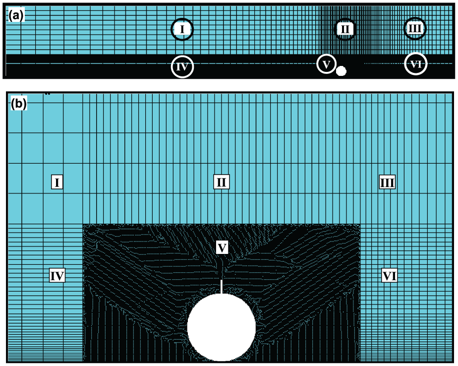
(a) The whole mesh system and (b) local mesh around the pipe.

The number of cells in subdomains, where the flow is unaffected or slightly affected by the presence of the cylinder, was 40 × 10, 40 × 10, 40 × 10, 40 × 40, and 40 × 40 for subdomains I, II, III, IV, and VI, respectively. The shape of elements used for these subdomains was rectangular. The meshes in subdomains I, III, IV, and VI were compressed in x direction toward the cylinder. Furthermore, compressed meshes were also used for subdomains IV and VI in y direction near the channel bed, and uniform mesh structure was used in subdomain II. As seen in Figure 2, finer meshes were used in subdomain V, where the flow is affected by the cylinder. Uniform triangular elements were used in this subdomain to prevent the amorphous structured elements near the cylinder due to the circular shape of the cylinder. Five different meshes were used to investigate the effect of mesh density on computational results by changing the density of mesh in subdomain V. The size of the elements in subdomain V was 4, 3, 2, 1, and 0.5 mm for Mesh 1, Mesh 2, Mesh 3, Mesh 4, and Mesh 5, respectively.

Near-wall treatment

The wall function and two-layer approaches were developed for modeling the nearby wall region. The processing time and the storage requirements for the solution of the problem can be significantly reduced using the wall function. Because in this approach, the first grid point near the wall is located outside the viscous sublayer for which the calculations of quantities are not required. The quantities at this first grid point are related to friction velocity based on the assumption of logarithmic velocity distribution. However, the use of wall functions in separated flows is questionable.⁴⁰

In two-layer approach, extremely fine grids are needed to resolve the viscous sublayer and the buffer layer. The first cell near the wall should be adjusted in the viscous sublayer where the linear viscous relations take place between the dimensionless velocity u⁺ = u/u_* and dimensionless distance y⁺ = u_*y/ν, where u_* (= (τ₀/ρ)^1/2) is friction velocity at the nearest wall, τ₀ is boundary stress, y is the distance from the wall, and ν is the kinematic viscosity of the fluid. Past observations^30,35,41 indicated that the value of the non-dimensional distance from the wall dominated by viscous shear is varied about y⁺=20–40. Akoz et al.³⁵ limited the viscosity-affected region using the value of y⁺=30 as a criterion to evaluate the adequacy of the mesh size nearby the bed with no-slip condition. On this basis, the size of the wall of an adjacent cell was adjusted for the two-layer model. The values of y⁺ for the different meshes used in this study are given in Table 1. As can be seen from Table 1 that Meshes 3, 4, and 5 are found to be adequate since the values of y⁺ remain below 30 as suggested by previous researchers.^30,35,41

Table 1.

Values of y⁺ (u_*y/u) for different computational mesh sizes.

Mesh no.	Size of the elements in subdomain V (mm)	Maximum y⁺ (u_*y/u)
1	4	46.2
2	3	34.5
3	2	26.0
4	1	10.3
5	0.5	8.067

Two-layer approaches with the mixing-length modification scheme of Van Driest⁴² is used with no-slip boundary condition in the study. Van Driest⁴² modified the mixing length, $(ℓ = κ y)$ , by a damping function as

ℓ = κ y [1 - \exp (- \frac{y^{+}}{A})]

(5)

In equation (5), κ is the von Kármán constant (κ = 0.4) and A is constant (A = 26).

Mesh independence was achieved by comparing the velocity distributions of numerical and experimental results at (N = 8) points on a line located equally spaced at the gap between the bed and pipe for G = 10 mm. Also, the turbulence closure models are compared using the root mean square error (RMSE) criterion which is given in Table 2. RMSE is defined as follows

RMSE = \sqrt{\frac{1}{N} \sum_{n = 1}^{N} \frac{1}{u_{0}^{2}} {(u_{n}^{m} - u_{n}^{p})}^{2}}

(6)

Table 2.

Mean square error statistics for different turbulence closure models on different computational meshes.

Mesh no.	Turbulence model
Mesh no.	k–ε	k–ω	SST
1	0.004316	0.004616	0.004909
2	0.001921	0.00211	0.002413
3	0.001016	0.000455	0.001271
4	0.000333	0.000319	0.000462
5	0.000318	0.000309	0.000445

SST: shear stress transport.

In equation (6), N is the total number of data and $u_{n}^{m}$ is the measured and $u_{n}^{p}$ is the predicted horizontal velocities. As seen in Table 2, the lowest value of RMSE is 0.000309 on Mesh 5 for k–ω turbulence closure model. The results presented in Table 2 show that the values of RMSE found on Mesh 4 are not much different than those of Mesh 5. The data presented in Tables 1 and 2 show that the results obtained from Mesh 4 and Mesh 5 are found to be similar. On the other hand, the required CPU time is increased for Mesh 5 approximately four times in comparison to Mesh 4. Therefore, it can be concluded that the Mesh 4 is fine enough to ensure that the results obtained are not mesh dependent. Thus, Mesh 4 was used as the computational mesh in the evaluation of the numerical results

Numerical results

As with the results of Akoz et al.,³⁵ the flow fields around the cylinder computed by k–ω and SST turbulence closure models are found to be similar to each other. Therefore, in sections “Streamlines” and “Velocity distribution in the gap,” the computational time–averaged velocity fields obtained using only the k–ω and the k–ε turbulence models on Mesh 4 are given and compared with the experimental results of Öner.²⁸

Streamlines

Figure 3 shows a comparison between the streamline patterns of a flow around a cylinder with and without spoiler at Re_D = 9500 for different gap ratios obtained by particle image velocimetry (PIV) technique, reported by Öner.²⁸ As can be seen from Figure 3, attaching a spoiler on a pipe caused the stagnation point to move upward due to the increase in size of the upstream separation region. In addition, the extension of separation zones at the upstream and downstream side of the cylinder will augment the concentration of the vorticity, thus speeding up the scouring process.²⁸

Figure 3.

Experimental time-averaged patterns (obtained by means of PIV) of streamlines for pipeline without (left column) and with spoiler (right column).^7,28

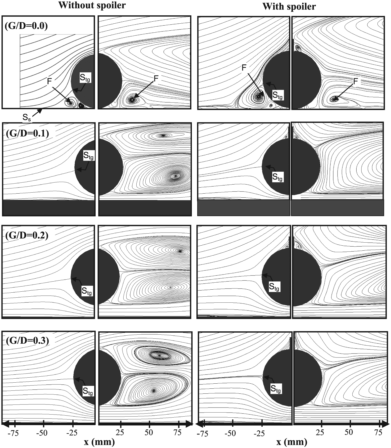
As can be seen from the streamlines given in Figure 3, there is a primary separation zone adjoining the pipe at the upstream side of the cylinder and a large separation zone with a secondary region between the pipe and bed for G/D = 0.0 with and without spoiler. It can be observed from Figure 3 that the presence of a spoiler increases the size of the separation zones. In addition, for a pipe lying on the bed, the initial point of separation zone, Ss; upward and downward faces of the cylinder; and a well-defined focus points, F, can be clearly seen from the experimental results given in Figure 3. Unfortunately, the focus points of the wake cannot be seen from the measured flow area for G/D = 0.0. In Figure 3, for G/D = 0.1, the upstream separation zone tends to disappear, regardless of the presence of spoiler. For G/D = 0.2, there is no upstream separation zone for the cylinder without spoiler. On the other hand, the separation region reserves its existence at the upstream side of the cylinder with spoiler. Similar observation can be made for G/D = 0.3 from Figure 3.

Figure 4 shows the simulated time–averaged streamline patterns of flow around a pipe without and with spoiler that is mounted on the bed (G/D = 0.0) using k–ε and k–ω turbulence models for Re_D = 9500. It can be seen from Figure 4 that for a pipe without a spoiler, there is a primary separation zone at the upstream side of the pipe, and on the downstream side, there is a large separation region with a secondary separation zone adjoining the pipe. Also, in Figure 4, agreeable with the experimental results given in Figure 3, when the spoiler was attached on top of the pipe the size of the separation zones increases. This expansion of the separation regions moved the stagnation point to an upward direction. It can be observed from Figure 4 that the simulated initial point of separation zone, S_s, and the focus points of the separation areas agree quite well with the measured flow results reported by Öner.²⁸ It can also be observed from Figure 4 that the separation zones, both at the upstream and downstream sides of the cylinder, obtained by k–ε are relatively smaller in size than those predicted by k–ω.

Figure 4.

Computational time–averaged streamlines of flow around a cylinder without and with spoiler using: (a) k–ε and (b) k–ω turbulence models at G/D = 0.0.

The simulated time–averaged streamline patterns of flow around a pipe without and with spoiler at G/D = 0.1 are presented in Figure 5. It is clearly seen from Figure 5 that a saddle point (S_p) and focus points of the wake occur at the downstream of the pipeline. Moreover, it is also observed that the boundary layer separates from the wall on the downstream side of the cylinder and forms a separation zone with a clear focus point. Figure 5 shows that the upstream separation region tends to disappear, except for the pipe with spoiler computed by k–ω turbulence closure model. It is observed from Figure 5 that the sizes of the separation zones obtained by k–ε turbulence model get smaller similar to Figure 4.

Figure 5.

Computational time–averaged streamlines of flow around a cylinder without and with spoiler using: (a) k–ε and (b) k–ω turbulence models at G/D = 0.1.

The computed time–averaged streamline patterns of flow area for G/D = 0.2 are presented in Figure 6. For this gap ratio, the flow area resembles the flow around an isolated pipe without a spoiler case. However, when the spoiler is mounted on the cylinder, the upstream separation region and the wall boundary separation at the downstream side of the cylinder occur and the computed sizes of the separation regions obtained by k–ε model gets smaller, similar to observation made from Figures 4 and 5.

Figure 6.

Computational time–averaged streamlines of flow around a cylinder without and with spoiler using: (a) k–ε and (b) k–ω turbulence models at G/D = 0.2.

The time-averaged streamline patterns of the computed flow area for G/D = 0.3 is given in Figure 7. Figure 7 shows that the effect of wall boundary on the flow around the cylinder decreases as the gap increases, and the flow area around the pipe without spoiler looks like to an isolated pipeline for this gap ratio. No separation region occurs on the bed neither on the upstream nor on the downstream of the pipe. Figures 4 –7 show that agreeable with the experimental results, attaching a spoiler on a pipe increases the size of the upstream separation zone and this caused the stagnation point to move to an upward position. It is obvious that the movement of the stagnation point angle due to the presence of the spoiler caused a change in the drag and the lift forces.

Figure 7.

Computational time–averaged streamlines of flow around a cylinder without and with spoiler using: (a) k–ε and (b) k–ω turbulence models at G/D = 0.3.

Velocity distribution in the gap

The comparison of time-averaged computed and measured horizontal and vertical velocity distributions at different locations of gap flow for a pipe with spoiler is shown in Figure 8.

Figure 8.

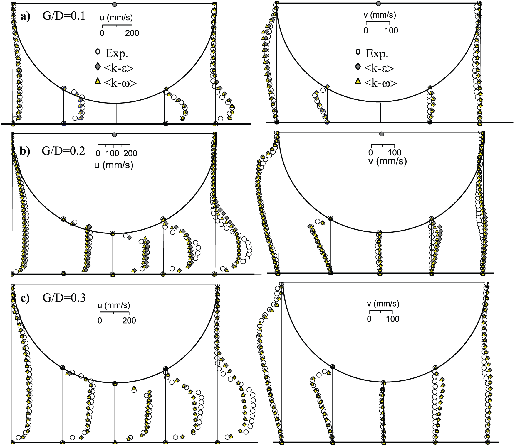
Horizontal and vertical velocity distributions of computed and measured flow at different locations of gap: (a) G/D = 0.1, (b) G/D = 0.2 and (c) G/D = 0.3, with spoiler.

Figure 8 shows that the general computed horizontal and vertical velocity distributions of the gap flow looked similar to measured velocity distributions. However, it seems that numerical velocity distributions obtained by k–ω turbulence model provide slightly better predictions than k–ε model.

Force coefficients

The comparisons of computed and measured results confirm that the computations using the k–ω turbulence model on Mesh 4 predict the flow around a pipe with and without spoiler well. Therefore, in this section, the drag and lift coefficients for the force on the pipe with and without spoiler computed using k–ω on Mesh 4 is presented and compared with the experimental results of Cheng and Chew²⁷ and Choi and Lee.³ The drag and lift coefficients C_D and C_L are given as follows

C_{D} = \frac{F_{D}}{ρ u_{o}^{2} D / 2}

(7)

C_{L} = \frac{F_{L}}{ρ u_{o}^{2} D / 2}

(8)

The drag and lift forces (F_D and F_L per unit length on the cylinder) in equations (7) and (8) were calculated as follows

F_{D} = \int_{0}^{2 π} (p \cos θ + τ_{0} \sin θ) rd θ

(9)

F_{L} = \int_{0}^{2 π} (- p \sin θ + τ_{0} \cos θ) rd θ

(10)

In equations (9) and (10), p is the pressure, τ₀ is the shear stress on the cylinder surface, and θ is the angle of the axis of the cylinder in clockwise direction.

Zdravkovich² and Lei et al.⁸ reported that in artificial thick boundary layers, there was a negative downward lift force acting on the pipe. Also, it is known that attaching a spoiler on the top of a pipe causes the force coefficient of drag force to increase and lift force coefficient to decrease.^24,27,43 The decrease in the lift coefficient caused a downward force. Bijker⁴³ reported that this reversed hydrodynamic lift force pushes and pulls the pipe downward. Thus, the downward lift force caused by the presence of the spoiler on top of the pipe seems to be one of the most important parameters of the self-burial process.

Figure 9 presents the change in computed drag coefficients with G/D for a pipe with and without spoiler. Figure 9 shows that in contrast to indications of Cheng and Chew²⁷ that the addition of the spoiler increases the drag coefficient, C_D, significantly for all gap ratios considered in their study, the value of the drag coefficient is found to be smaller for G/D = 0.0, and it is almost equal to the value obtained without a spoiler case for G/D = 0.1 in this study. However, a close observation from Figure 9 shows that the addition of a spoiler on top of a pipe increases the drag coefficient on pipe similar to observations made in the past^2,24,27,43 for G/D > 0.1. The simulated results given in Figure 9 show that the general trend in increasing the drag coefficient of the pipe is found to be similar to the past studies.^2,24,27,43 However, the values of the drag coefficients with and without spoiler cases obtained in this study were found to be smaller than those of the past observations.^2,24,27,43 Different results about drag coefficient can be found in the literature particularly for pipes without spoiler. For instance, Cheng and Chew²⁷ reported that their numerical predictions overestimated the drag coefficient for a single pipe case. They claimed that three-dimensional (3D) effect was the main reason for the difference between experimental and numerical results as it was explained by Lei.⁴⁴ Lei⁴⁴ reported that the value of predicted drag coefficient by a 3D model was about 1.1, while the 2D model gave 1.45. The reasons for the differences between results obtained for the drag coefficient in the literature may be various; these are flow conditions, experimental or numerical methods, diameter of the pipe, gap ratio (G/D), and so on.

Figure 9.

Comparisons of the computed drag coefficients between this study, with and without spoiler, and observations of Zdravkovich² and Choi and Lee³ for gap ratio without spoiler case.

Figure 10 shows the computed lift coefficients versus different gap ratios without spoiler case and the computed results obtained from this study compared with the observations of Cheng and Chew²⁷ and Choi and Lee.³ It is seen from Figure 10 that the lift coefficient decreases as the gap ratio increases. This is mainly due to the effect of boundary layer and the separation areas occurred at upstream of the pipe that caused the stagnation point to move upward position and also the suppression of vortex shedding for small gap ratios. Figure 10 indicates favorable agreements between the results reported by Cheng and Chew,²⁷ Choi and Lee,³ and computational results of this study. Kazeminezhad et al.’s³⁸ observations also confirmed the results of this study. Kazeminezhad et al.³⁸ obtained the lift coefficient for G/D = 0.0 as a value between 0.6 and 0.83. Kazeminezhad et al.³⁸ also reported that the C_L was increased as the thickness of the boundary layer decreased, particularly for the smaller gap ratios.

Figure 10.

Comparisons of the computed lift coefficients between this study and results of Cheng and Chew²⁷ and Choi and Lee³ for gap ratio without spoiler case.

Figure 11 illustrates the computed lift coefficients versus gap ratio and compares them with the results of Cheng and Chew²⁷ obtained for different spoiler lengths and Reynolds numbers. The present computed results are in good agreement with the observations of Cheng and Chew.²⁷ As can be seen from Figure 11, attachment of a spoiler on top of a pipe decreases the lift coefficient. Furthermore, C_L has negative values in the presence of the spoiler, and this depicts a non-zero downward lift. Cheng and Chew²⁷ reported that the increase in the pressure between θ = 0° and 90° and the decrease in the pressure between θ = 90° and 180° are the main reasons for the non-zero downward lift acting on the pipe.

Figure 11.

Comparisons of the computed lift coefficients between this study (Re_D = 9500) and observations of Cheng and Chew²⁷ for different spoiler sizes and different Re numbers for gap ratio with spoiler case.

Conclusion

In this study, the flow around a near-bed pipeline with a spoiler has been simulated at Re = 9500. The Reynolds-averaged Navier–Stokes equations with k–ε, k–ω, and SST turbulence closure models have been employed to investigate the effect of spoiler on streamline patterns, on velocity distributions passing through the gap between the pipe and the bed, and on the force coefficients. The computed results were compared with experimental and numerical data given in the past.^{2,3,7,27–29} As a result, the following conclusions were made from the study:

The separation zones obtained by k–ε are relatively smaller in size compared to those predicted by means of the k–ω and the SST models. This can be explained by the fact that the k–ε turbulence closure model has difficulties to simulate accurately the flow area in the presence of adverse pressure gradient boundary layer flow, therefore it does not predict the onset of separation accurately.³⁴

Computational results of horizontal and vertical velocity distributions of the gap flow obtained using k–ω and k–ε turbulence models are found to be in agreement with the measured results. Besides, velocity distributions obtained by k–ω turbulence model provide slightly better prediction results than those of k–ε model.

The comparisons of the numerical and experimental results show that the k–ω turbulence closure model on the best mesh design predicts the flow around a pipe with and without spoiler well.

C_L coefficient decreases as the gap increases for a pipe without spoiler. The present computations show that the values of C_L are 0.63, 0.2442, 0.1801, and 0.1339 for a pipeline without spoiler at G/D = 0.0, 0.1, 0.2, and 0.3, respectively, whereas for a pipeline with a height of 0.2D spoiler the values are −0.018, −0.319, −0.53, and −0.788. The computations show that attaching a spoiler on the pipe caused C_L to have negative values, which depicts a non-zero downward lift which forced the pipeline downward.

As a summary, based on the results obtained from this study, the self-burial process of the pipeline on the seabed can be explained as follows. When a spoiler is mounted on a pipe, more energetic vorticity regions are formed in both upstream and downstream sides of the pipe resulting in speeding up seepage transpiring on the seabed and thus increasing the intensity and amount of scours.

It is clear that this process stimulates the scouring mechanism and decreases the bearing capacity of the seabed, and then, the downward lift force pushes the pipeline into the seabed resulting in “self-burial” of the pipeline.

Footnotes

Academic Editor: Pietro Scandura

Declaration of conflicting interests

The author(s) declared no potential conflicts of interest with respect to the research, authorship, and/or publication of this article.

Funding

The author(s) disclosed receipt of the following financial support for the research, authorship, and/or publication of this article: This work was supported by the Scientific and Technological Research Council of Turkey through Project 107M641.

References

Bearman

Zdravkovich

MM.

Flow around a circular cylinder near a plane boundary. J Fluid Mech 1978; 89: 33–47.

Zdravkovich

MM.

Forces on a circular cylinder near a plane wall. Appl Ocean Res 1985; 7: 197–201.

Choi

Lee

SJ.

Ground effect of flow around an elliptic cylinder in a turbulent boundary layer. J Fluid Struct 2000; 14: 697–709.

Price

Sumner

Smith

. Flow visualization around a circular cylinder near to a plane wall. J Fluid Struct 2002; 16: 175–191.

Zdravkovich

MM.

Flow around circular cylinders, vol. 1: fundamentals. New York: Oxford University Press Inc, 1997.

Öner

Kırkgöz

MS.

Düzenli akımda tabana yakın yatay silindir yüzeyinde ve tabanda kayma gerilmesi dağılımlarının deneysel incelenmesi. ÇÜ Müh Mim Fak Dergisi 2007; 22: 93–105.

Öner

Kırkgöz

Aköz

MS.

Interaction of a current with a circular cylinder near a rigid bed. Ocean Eng 2008; 35: 1492–1504.

Lei

Cheng

Kavanagh

Re-examination of the effect of a plane boundary on force and vortex shedding of a circular cylinder. J Wind Eng Ind Aerod 1999; 80: 263–286.

Zovatto

Pedrizzetti

Flow about a circular cylinder between parallel walls. J Fluid Mech 2001; 440: 1–25.

10.

Liang

Cheng

. Numerical modeling of flow and scour below a pipeline in currents: part I. Flow simulation. Coast Eng 2005; 52: 25–42.

11.

Kırkgöz

Öner

AA.

Yatay bir dairesel silindir etrafındaki akımda hız alanının deneysel ve teorik incelenmesi. ÇÜ Müh Mim Fak Dergisi 2006; 21: 85–98.

12.

Aköz

M S

Öner

A A

Kırkgöz

M S.

Tabana yakın bir silindir etrafındaki akımın farklı türbülans modelleri ile sayısal modellenmesi. ÇÜ Müh Mim Fak Dergisi 2007; 22: 107–117.

13.

Mao

. Seabed scours under pipelines. In: Proceedings of the seventh international conference on offshore mechanics and arctic engineering, ASME, Houston, TX, 7–12 February 1988, pp.33–38.

14.

Chiew

YM.

Mechanics of local scour around submarine pipelines. J Hydraul Eng: ASCE 1990; 116: 515–529.

15.

Sumer

Fredsoe

Onset of scour below pipelines exposed to waves. Int J Offshore Polar 1991; 1: 189–194.

16.

Klomp

WHG

Hansen

Chen

. Pipeline seabed interaction, free span development. In: Proceedings of the fifth international offshore and polar engineering conference, The Hague, 11–16 June 1995, pp.117–122. Mountain View, CA: ISOPE.

17.

Dey

Singh

Clear water scour below underwater pipelines. J Hydro Res 2007; 1: 157–162.

18.

Zang

Cheng

Zhao

. A numerical model for onset of scour below offshore pipelines. Coast Eng 2009; 56: 458–466.

19.

Cheng

Yeow

Zhang

. Three dimensional scour below offshore pipelines in steady currents. Coast Eng 2009; 56: 577–590.

20.

Gao

Luo

Flow-pipe-seepage coupling analysis of spanning initiation of partially-embedded pipeline. J Hydrodyn 2010; 22: 478–487.

21.

Arya

Shingan

Scour-mechanism, detection and mitigation for subsea pipeline integrity. Int J Eng Res Technaol 2012; 1: 1–14.

22.

Hulsbergen

. Simulated self-burial of submarine pipelines. In: Offshore technology conference, Houston, TX, 7–9 May 1984, OTC-4667, pp.171–178. Houston, TX: Offshore Technology Conference.

23.

Hulsbergen

. Spoilers for stimulated self-burial of submarine pipelines. In: Offshore technology conference, Houston, TX, 5–8 May 1986, OTC-5339, pp.441–444. Houston, TX: Offshore Technology Conference.

24.

Hulsbergen

Bijker

. Effect of spoilers on submarine pipeline stability. In: Offshore technology conference, Houston, TX, 1–4 May 1989, OTC-4467, pp.171–178. Houston, TX: Offshore Technology Conference.

25.

Chiew

YM.

Effect of spoilers on scour at submarine pipelines. J Hydraul Eng: ASCE 1992; 118: 1311–1317.

26.

Chiew

YM.

Effect of spoilers on wave-induced scour at submarine pipelines. Coast Ocean Eng 1993; 119: 417–428.

27.

Cheng

Chew

LW.

Modeling of flow around a near bed pipeline with spoiler. Ocean Eng 2003; 30: 1595–1611.

28.

Öner

AA.

The flow around a pipeline with a spoiler. Proc IMechE, Part C: J Mechanical Engineering Science 2009; 224: 109–121.

29.

Öner

Kırkgoz

MS.

Experimental study of shear stress distributions on the surface of near-bed horizontal cylinder and on the bed in steady flow. ÇUJ Fac Eng Arch 2007; 22: 93–105.

30.

White

FM.

Viscous fluid flow. Singapore: McGraw-Hill, 1991.

31.

Wilcox

DC.

Turbulence modeling for CFD. La Cañada, CA: DCW Industries, Inc, 2000.

32.

Launder

Spalding

DB.

The numerical computation of turbulent flows. Comput Method Appl M 1974; 3: 269–289.

33.

Wilcox

DC.

Reassessment of the scale-determining equation for advanced turbulence models. AIAA J 1988; 26: 1299–1310.

34.

Menter

FR.

Two-equation eddy-viscosity turbulence models for engineering applications. AIAA J 1994; 32: 1598–1605.

35.

Akoz

Kirkgoz

Öner

AA.

Experimental and numerical modeling of a sluice gate flow. J Hydraul Res 2009; 47: 167–176.

36.

Kırkgöz

Aköz

Öner

AA.

Numerical modeling of flow over a chute spillway. J Hydraul Res 2009; 47: 790–797.

37.

Aköz

Kırkgöz

MS.

Numerical and experimental analyses of the flow around a horizontal wall-mounted circular cylinder. T Can Soc Mech Eng 2009; 33: 189–216.

38.

Kazeminezhad

Yeganeh-Bakhtiary

Etemad-Shahidi

Numerical investigation of boundary layer effects on vortex shedding frequency and forces acting upon marine pipeline. Appl Ocean Res 2010; 32: 460–470.

39.

Dayem

Bayomi

NN.

Experimental and numerical flow visualization of a single square cylinder. Int J Comp Meth Eng Sci Mech 2006; 7: 113–127.

40.

Rodi

Comparison of LES and RANS calculations of the flow around bluff bodies. J Wind Eng Ind Aerod 1997; 69–71: 55–75.

41.

Kırkgöz

Ardiclioglu

Velocity profiles of developing and developed open channel flow. J Hydr Eng 1997; 123: 1099–1105.

42.

Van Driest

. On turbulent flow near a wall. J Aeron Sci 1956; 23: 1007–1011.

43.

Bijker

Achieving sub-sea pipeline burial and stability with spoilers. Pipeline Gas J 2000; 227: 46.

44.

Lei

Experimental and numerical studies of vortex shedding flow over a circular cylinder near a wall. PhD Thesis, Department of Civil and Resource Engineering, The University of Western Australia, Perth, WA, Australia, 1999.

Numerical investigation of flow around a pipeline with a spoiler near a rigid bed

Abstract

Keywords

Introduction

Governing equations

Numerical method and solution domain

Numerical method

Solution domain and boundary conditions

Computational meshing

Near-wall treatment

Numerical results

Streamlines

Velocity distribution in the gap

Force coefficients

Conclusion

Footnotes

Declaration of conflicting interests

Funding

References