Sage Journals: Discover world-class research

Abstract

In the long-term service period, the bridge health monitoring system produced a huge amount of monitoring stress data; proper handling of these data is one of the main difficulties in the field of structural health monitoring, especially to predict the structural stress based on the monitored data. The objectives of this article are to present: (1) a nonlinear dynamic model, (2) a nonlinear mixed Gaussian particle filtering algorithm for predicting the monitored data based on the dynamic model, and (3) an approach combining nonlinear mixed Gaussian particle filtering algorithm with structural health monitoring data to predict the structural stress under uncertainty in real time. And an actual example is provided to illustrate the application and feasibility of the proposed models and methods.

Keywords

Structural health monitoring a nonlinear dynamic model mixed Gaussian particle filtering algorithm prediction analysis uncertainty

Introduction

The past several decades have witnessed civil infrastructure design, assessment, and prediction shift from deterministic methodology to probabilistic methodology.¹ Structural health monitoring (SHM) develops so rapidly that it is likely to become a predominant emerging technology to challenge and improve traditional way of design, assessment, and prediction of civil infrastructure. The research on SHM generally experiences two stages. The first stage, falling in the mature stage, is to install sensors on the bridge structures and conduct much research on the data transition system, data acquisition technology, system integration technology, and other aspects.^2–4 The second stage is mainly the reasonable application of SHM data. A sound number of studies are mainly focused on the modal parameter identification, structural damage detection, performance prediction, and reliability assessment. Novel monitoring systems used in structural engineering contain sensors providing a large amount of monitored data (stress data). Proper handling of the continuously provided monitored data is one of the main difficulties in the SHM field for predicting stress data.

SHM technologies, which are popularly used and extensively researched, are anticipated to be cost-effective. The SHM data should be utilized in reliability-based design, assessment, and prediction. There are great potentials to adopt these technologies into the rational performance prediction which is a key point for life-cycle reliability management.¹ For the research of bridge time-variant performance prediction and assessment, some achievements^5–16 are obtained, for instance, the reliability assessment of long-span truss bridge¹⁵ and the use of monitored extreme data in the structural performance prediction.¹⁶ But based on the bridges’ dynamic SHM data, the research on dynamically predicting the structural performance is at the initial stage in the world. Therefore, it is important and necessary to give applicable and essential method which integrates the real-time SHM data into the structural performance prediction.

To achieve the above goals, this article first builds the dynamic nonlinear model based on the SHM data. Then, the nonlinear mixed Gaussian particle filtering (MGPF) algorithm, which can be utilized to predict the structural monitored data in real time, is also first given based on the built dynamic nonlinear model. Finally, based on the real-time SHM data, the structural real-time performance is predicted with MGPF algorithm, and an actual example is provided to illustrate the application and feasibility of the proposed nonlinear model and the corresponding algorithm.

Dynamic nonlinear models based on SHM data

The dynamic nonlinear models usually include a nonlinear state equation, a linear observation equation, and the initial state information. The state equation shows changes of the system with time and reflects inner dynamic changes of the system and random disturbances. The observation equation expresses the relationship between the observed data and the current state parameters of the system. For each time t, the general dynamic nonlinear model is formally defined as follows:

Observation equation

y_{t + 1} = θ_{t + 1} + ν_{t + 1}, ν_{t + 1} ~ N [0, V_{t + 1}], (t = 1, 2, \dots, T)

(1)

State equation

θ_{t + 1} = h (θ_{t}) + ω_{t + 1}, ω_{t + 1} ~ N [0, W_{t + 1}], (t = 1, 2, \dots, T)

(2)

Initial information

(θ_{t} | D_{t}) ~ N [m_{t}, C_{t}] = f (θ_{t}) = \sum_{i = 1}^{n} p_{i} Φ (\frac{θ_{t} - μ_{i}}{σ_{i}})

(3)

where, y_t +₁ is the observation data at time t + 1, $ν_{t + 1}$ is the observation error or the observation noise at time t + 1, $θ_{t + 1}$ is the state variable at time t + 1, $N [\cdot]$ is normal probability density function (PDF), V_t_+ 1 is the variance which indicates the uncertainty of observation errors, $h (\cdot)$ is nonlinear function, and W_t +₁ is the variance which indicates the model uncertainty recursive from time t to time t + 1. $ω_{t + 1}$ is the state error or state noise at time t + 1, T is the monitored total time, and the initial information is the probabilistic representation of the predictors’ belief about the level $θ_{t}$ at time t. The mean value $m_{t}$ is a point estimate of this level $θ_{t}$ , and $C_{t}$ measures the associated uncertainty. Each information set $D_{t}$ comprises all the information available at time t, including $D_{0}$ , the values of the variances ${V_{t + 1}, W_{t + 1} : t > 0}$ , and the values of the observations $y_{t - 1}, y_{t - 2}, \dots, y_{1}$ . Thus, the only new information becoming available at time t is the observational value $y_{t}$ , so $D_{t} = {y_{t}, D_{t - 1}}$ .

For the long-term performance prediction of bridge structures, the nonlinear dynamic model has the better prediction precision than the dynamic linear model^6,10,12 which is mainly for short-term prediction of monitored data, so the dynamic nonlinear model is adopted to predict the performance data (stress and reliability indices) of bridge. In this article, for the long-term health monitoring data, the quadratic function model can be approximately and reasonably adopted to build the state equation. The dynamic nonlinear model is built as follows.

The quadratic function

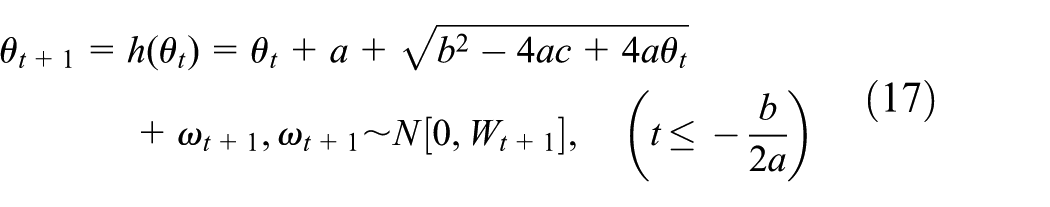
For the long-term health monitored data of bridges, the h(t) (fitted quadratic function) is commonly well fitted to show the changing trend of the monitored data; therefore, h(t) can be approximately and reasonably considered as the changing curves of state data or trend data, which are expressed as

h (t) = a t^{2} + bt + c

(4)

θ_{t} = h (t) = a t^{2} + bt + c

(5)

θ_{t + 1} = h (t + 1) = a (t + 1)^{2} + b (t + 1) + c

(6)

where a, b, and c are all regression coefficients of monitored data. $t = time$ , the unit of which is day. $θ_{t}$ is the state data at time t.

Based on equation (5)

a t^{2} + bt + c - θ_{t} = 0

(7)

The solutions of equation (7) are

t_{2}^{1} = \frac{- b \pm \sqrt{b^{2} - 4 a (c - θ_{t})}}{2 a}

(8)

Based on equation (6)

a t^{2} + (2 a + b) t + a + b + c - θ_{t + 1} = 0

(9)

The solutions of equation (9) are

t_{2}^{1} = \frac{- b - 2 a \pm \sqrt{{(2 a + b)}^{2} - 4 a (a + b + c - θ_{t + 1})}}{2 a}

(10)

The transformed approximate state equation based on quadratic function

With equations (8) and (10), for $t \geq 0$ , considering the consistency and equality of the solutions, there are

\begin{matrix} \frac{- b \pm \sqrt{b^{2} - 4 a (c - θ_{t})}}{2 a} \\ = \frac{- b - 2 a \pm \sqrt{{(2 a + b)}^{2} - 4 a (a + b + c - θ_{t + 1})}}{2 a} \end{matrix}

(11)

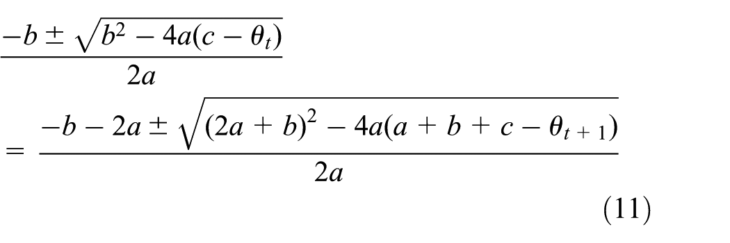
After equation (11) is simplified, the transferred approximate state equation can be obtained as the follows:

If $a > 0$ , then the state equations are

\begin{matrix} θ_{t + 1} = h (θ_{t}) = θ_{t} + a + \sqrt{b^{2} - 4 ac + 4 a θ_{t}}, \\ (t \leq - \frac{b}{2 a}) \end{matrix}

(12)

and

\begin{matrix} θ_{t + 1} = h (θ_{t}) = θ_{t} + a - \sqrt{b^{2} - 4 ac + 4 a θ_{t}}, \\ (t > - \frac{b}{2 a}) \end{matrix}

(13)

If $a < 0$ , then the state equations are

\begin{matrix} θ_{t + 1} = h (θ_{t}) = θ_{t} + a - \sqrt{b^{2} - 4 ac + 4 a θ_{t}}, \\ (t \leq - \frac{b}{2 a}) \end{matrix}

(14)

and

\begin{matrix} θ_{t + 1} = h (θ_{t}) = θ_{t} + a + \sqrt{b^{2} - 4 ac + 4 a θ_{t}}, \\ (t > - \frac{b}{2 a}) \end{matrix}

(15)

where equations (12)–(15) show that the approximate state equations exist two different cases, namely, equations (12) and (13) and equations (14) and (15). The case, which is more reasonable, accurate, and applicable, depends on the regressive coefficients (a, b, and c) and the state parameter $θ_{t}$ .

The dynamic nonlinear model

Based on section “The transformed approximate state equation based on quadratic function,” considering the uncertainty of observation variable and state variable, the built dynamic nonlinear models in this article are explained as follows

Observation equation is

y_{t + 1} = θ_{t + 1} + ν_{t + 1}, ν_{t + 1} ~ N [0, V_{t + 1}], (t = 1, 2, \dots, T)

(16)

If $a > 0$ , then the state equations are

\begin{matrix} θ_{t + 1} = h (θ_{t}) = θ_{t} + a + \sqrt{b^{2} - 4 ac + 4 a θ_{t}} \\ + ω_{t + 1}, ω_{t + 1} ~ N [0, W_{t + 1}], (t \leq - \frac{b}{2 a}) \end{matrix}

(17)

and

\begin{matrix} θ_{t + 1} = h (θ_{t}) = θ_{t} + a - \sqrt{b^{2} - 4 ac + 4 a θ_{t}} + ω_{t + 1}, \\ ω_{t + 1} ~ N [0, W_{t + 1}], (t > - \frac{b}{2 a}) \end{matrix}

(18)

If $a < 0$ , then the state equations are

\begin{matrix} θ_{t + 1} = h (θ_{t}) = θ_{t} + a - \sqrt{b^{2} - 4 ac + 4 a θ_{t}} + ω_{t + 1}, \\ ω_{t + 1} ~ N [0, W_{t + 1}], (t \leq - \frac{b}{2 a}) \end{matrix}

(19)

and

\begin{matrix} θ_{t + 1} = h (θ_{t}) = θ_{t} + a + \sqrt{b^{2} - 4 ac + 4 a θ_{t}} + ω_{t + 1}, \\ ω_{t + 1} ~ N [0, W_{t + 1}], (t > - \frac{b}{2 a}) \end{matrix}

(20)

Initial state information is

(θ_{t} | D_{t}) ~ N [m_{t}, C_{t}] = f (θ_{t}) = \sum_{i = 1}^{n} p_{i} Φ (\frac{θ_{t} - μ_{i}}{σ_{i}})

(21)

where, a, b, and c are constants, and $θ_{t}$ is the state parameter indicating the level of the observational data at time t.

Determination of the main probability parameters of dynamic nonlinear models

For the dynamic nonlinear model, the main probability parameters are V_t_+ 1, W_t_+ 1, m_t, and C_t. The method of determining the main probability parameters is as follows.

In this article, the interval period of model updating is 1 day; V_t_+ 1 is estimated with the variance of differences between resampled data and monitored data. W_t_+ 1 can be estimated with the variance of differences between resampled data and the fitted changing trend data.

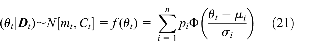
$m_{t}$ is the mean value of state variable at time t; $C_{t}$ is the variance of state variable at time t. They can be both estimated with the smoothly processed or resampled monitored data at time t and before time t. The steps are as follows:

1. With estimation method of kernel density, the actual distribution function $G (θ_{t})$ of the initial state data (smoothly processed or resampled monitored data) is approximately $g (θ_{t})$ , namely

G (θ_{t}) \approx g (θ_{t})

(22)

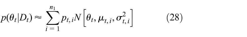
2. Since any set of data can be fitted by a few normal distributions, namely

G (θ_{t}) \approx \sum_{i = 1}^{n} p_{i} Φ (\frac{θ_{t} - μ_{i}}{σ_{i}})

(23)

where $\sum_{i = 1}^{n} p_{i} = 1$ and $p_{i} \geq 0$ , and $Φ (\cdot)$ denotes the cumulative probability distribution functions of standard normal distribution.

3. The weights and distribution parameters of the fitted normal distributions can be obtained with the least residual error quadratic sum method OLS, namely

OLS = \sqrt{\frac{1}{n} \sum_{j = 1}^{k} {(g (θ_{t}) - (\sum_{i = 1}^{n} p_{i} Φ (\frac{θ_{t} - μ_{i}}{σ_{i}})))}^{2}}

(24)

where $p_{i}$ is the weight. The values of unknown parameters for the fitted distributions can be possessed by the optimization computation with the rule of OLS. Furthermore, the optimized parameters must be determined to make sure that the value of OLS is the minimum.

MGPF algorithm based on the nonlinear dynamic model

Based on the built dynamic nonlinear models shown in equations (16)–(21), with Bayesian method and conditional probability method, the following can be reached.

Priori probability distribution $p (θ_{t + 1} | D_{t})$ of state $θ_{t + 1}$

p (θ_{t + 1} | D_{t}) = \int p (θ_{t + 1} | θ_{t}) p (θ_{t} | D_{t}) d θ_{t}

(25)

where $p (θ_{t + 1} | θ_{t})$ can be computed with equations (17)–(21), $p (θ_{t} | D_{t})$ can be approximately obtained with equation (21).

One-step forward ahead prediction distribution $p (y_{t + 1} | D_{t})$

p (y_{t + 1} | D_{t}) = \int p (θ_{t + 1} | D_{t}) p (y_{t + 1} | θ_{t + 1}) d θ_{t + 1}

(26)

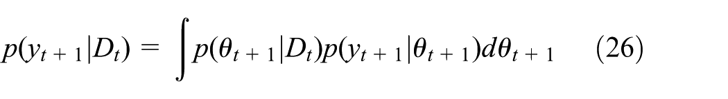
where $p (y_{t + 1} | θ_{t + 1})$ can be computed with equations (16) and (25).

Posteriori probability distribution $p (θ_{t + 1} | D_{t + 1})$ of state $θ_{t + 1}$

p (θ_{t + 1} | D_{t + 1}) = \frac{p (θ_{t + 1} | D_{t}) p (y_{t + 1} | θ_{t + 1})}{p (y_{t + 1} | D_{t})}

(27)

The approximate PDF (importance function) of $p (θ_{t + 1} | D_{t + 1})$ based on the extended Kalman filter

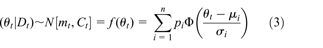
Based on equation (21), PDF of the initial state information at time t can be obtained as follows

p (θ_{t} | D_{t}) \approx \sum_{i = 1}^{n_{1}} p_{t, i} N [θ_{t}, μ_{t, i}, σ_{t, i}^{2}]

(28)

where $p_{t, i}$ is the weight of the ith normal PDF $N [θ_{t}, μ_{t, i}, σ_{t, i}^{2}]$ .

In this article, the observation error and state noise are both supposed to follow single normal distribution, so combining the state equation (equations (17)–(20)) with extended Kalman filter (EKF),¹⁷equation (25) can be further approximately transferred into

p (θ_{t + 1} | D_{t}) \approx \sum_{i = 1}^{n_{2}} {\bar{p}}_{t + 1, i} N [θ_{t + 1}, {\bar{μ}}_{t + 1, i}, {\bar{σ}}_{t + 1, i}^{2}]

(29)

where $\sum_{i = 1}^{n_{1}} p_{t, i} = \sum_{i = 1}^{n_{2}} {\bar{p}}_{t + 1, i} = 1$ and $p_{t, i}, {\bar{p}}_{t + 1, i} \geq 0$ , $N [\cdot]$ is normal PDF. The research¹⁸ shows that $n_{1} = n_{2}$

\begin{matrix} {\bar{μ}}_{t + 1, i} = h (μ_{t, i}); {\bar{σ}}_{t + 1, i}^{2} = {(H_{t + 1, i})}^{T} σ_{t, i}^{2} H_{t + 1, i} + W_{t + 1} \\ H_{t + 1, i} = \frac{\partial h (θ)}{\partial θ} |_{θ = μ_{t, i}}; p_{t, i} = {\bar{p}}_{t + 1, i} \end{matrix}

(30)

When y_t_+ 1 is obtained, based on equations (16) and (29), PDF $p (θ_{t + 1} | D_{t + 1})$ of state $θ_{t + 1}$ can be obtained as

p (θ_{t + 1} | D_{t + 1}) = C_{k} p (θ_{t + 1} | D_{t}) p (y_{t + 1} | θ_{t + 1})

(31)

where $C_{k} = \int p (θ_{t + 1} | D_{t}) p (y_{t + 1} | θ_{t + 1}) d θ_{t + 1}$ , with equations (29) and (31), the following can be reached

\begin{matrix} p (θ_{t + 1} | D_{t + 1}) \\ \approx C_{k} \sum_{i = 1}^{n_{2}} {\bar{p}}_{t + 1, i} p (y_{t + 1} | θ_{t + 1}) N [θ_{t + 1}, {\bar{μ}}_{t + 1, i}, {\bar{σ}}_{t + 1, i}^{2}] \\ \approx \sum_{i = 1}^{n_{2}} p_{t + 1, i} N [θ_{t + 1}, μ_{t + 1, i}, σ_{t + 1, i}^{2}] \end{matrix}

(32)

where

\begin{matrix} μ_{t + 1, i} = {\bar{μ}}_{t + 1, i} + K_{t + 1, i} ({y_{t}}_{+ 1} - {\bar{μ}}_{t + 1, i}), \\ σ_{t + 1, i}^{2} = {\bar{σ}}_{t + 1, i}^{2} - K_{t + 1, i} {\bar{σ}}_{t + 1, i}^{2} \\ K_{t + 1, i} = {\bar{σ}}_{t + 1, i}^{2} (V_{t + 1} + {\bar{σ}}_{t + 1, i}^{2})^{- 1}, \\ p_{t + 1, i} = \frac{{\bar{p}}_{t + 1, i} α_{t + 1, i}}{\sum_{i = 1}^{n_{2}} {\bar{p}}_{t + 1, i} α_{t + 1, i}}, \\ α_{t + 1, i} = N ({y_{t}}_{+ 1}, {\bar{μ}}_{t + 1, i}, V_{t + 1} + {\bar{σ}}_{t + 1, i}^{2}) \end{matrix}

(33)

The MGPF algorithm based on the nonlinear dynamic model

Based on equations (16)–(21) and (25)–(33), the MGPF algorithm based on the nonlinear dynamic model is shown as follows:

1. Posteriori probability distribution of the state at time t + 1 based on the Gaussian particles

Suppose that the priori PDF of $θ_{t + 1}$ is

p (θ_{t + 1} | D_{t}) \approx \sum_{i = 1}^{n_{2}} {\bar{p}}_{t + 1, i} N [θ_{t + 1}, {\bar{μ}}_{t + 1, i}, {\bar{σ}}_{t + 1, i}^{2}]

(34)

When y_t_+ 1 is obtained, with equation (32), the posteriori PDF $p (θ_{t + 1} | D_{t + 1})$ of $θ_{t + 1}$ can be approximately solved. The following is the recursive updating algorithm.

For $i = 1, \dots, n_{2}$ , sample M particles from the importance function $q_{i} (θ_{t + 1} | D_{t + 1})$ denoted by ${θ_{t + 1, i}^{m}}_{m = 1}^{M}$

q_{i} (θ_{t + 1} | D_{t + 1}) = N [θ_{t + 1}, μ_{t + 1, i}, σ_{t + 1, i}^{2}]

(35)

where $N [θ_{t + 1}, μ_{t + 1, i}, σ_{t + 1, i}^{2}]$ can be approximately obtained from equation (32).

For $i = 1, \dots, n_{2}$ and $m = 1, \dots, M$ , the each weight of the sampled particles is

r_{t + 1, i}^{m} = \frac{p (y_{t + 1} | θ_{t + 1, i}^{m}) N [θ_{t + 1} = θ_{t + 1, i}^{m} | {\bar{μ}}_{t + 1, i}, {\bar{σ}}_{t + 1, i}^{2}]}{q_{i} (θ_{t + 1, i}^{m} | D_{t + 1})}

(36)

Because $p (y_{t + 1} | θ_{t + 1}) N [θ_{t + 1}, {\bar{μ}}_{t + 1, i}, {\bar{σ}}_{t + 1, i}^{2}]$ is approximately Gaussian distribution,¹⁷ the sampled particles and the corresponding weights can be used to estimate the mean and variance, which are

μ_{t + 1, i} = \frac{\sum_{m = 1}^{M} (r_{t + 1, i}^{m} θ_{t + 1, i}^{m})}{\sum_{m = 1}^{M} r_{t + 1, i}^{m}}

(37)

\begin{matrix} σ_{t + 1, i}^{2} = \frac{\sum_{m = 1}^{M} r_{t + 1, i}^{m} (θ_{t + 1, i}^{m} - μ_{t + 1, i}) {(θ_{t + 1, i}^{m} - μ_{t + 1, i})}^{T}}{\sum_{m = 1}^{M} r_{t + 1, i}^{m}}, \\ i = 1, 2, \dots, n_{2} \end{matrix}

(38)

The updating of the particle weight

\begin{matrix} w_{t + 1, i} = {\bar{p}}_{t + 1, i} \frac{\sum_{m = 1}^{M} r_{t + 1, i}^{m}}{\sum_{i = 1}^{n_{2}} \sum_{m = 1}^{M} r_{t + 1, i}^{m}} |_{p_{t, i} = {\bar{p}}_{t + 1, i}}, \\ p_{t + 1, i} = \frac{w_{t + 1, i}}{\sum_{i = 1}^{n_{2}} w_{t + 1, i}} \end{matrix}

(39)

Finally, the posteriori PDF of $θ_{t + 1}$ is

p (θ_{t + 1} | D_{t + 1}) \approx \sum_{i = 1}^{n_{2}} p_{t + 1, i} N [θ_{t + 1}, μ_{t + 1, i}, σ_{t + 1, i}^{2}]

(40)

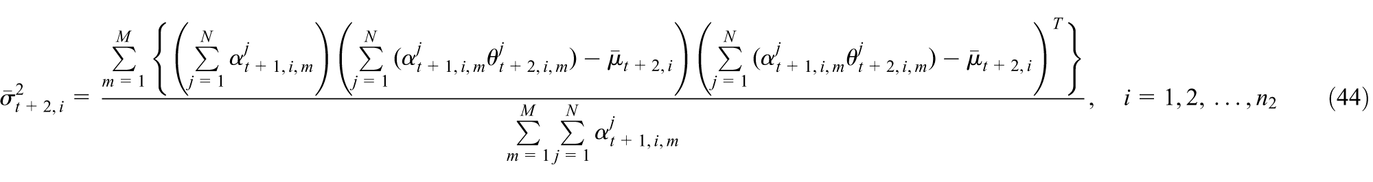
2. Priori probability distribution $p (θ_{t + 2} | D_{t + 1})$ of the state at time t + 2 based on the Gaussian particles

With equations (29), (34), and (40), the priori probability distribution of the state at time t + 2 $(p (θ_{t + 2} | D_{t + 1}))$ is given as

\begin{matrix} p (θ_{t + 2} | D_{t + 1}) \\ \approx \sum_{i = 1}^{n_{2}} p_{t + 1, i} \int N [θ_{t + 1}, μ_{t + 1, i}, σ_{t + 1, i}^{2}] p (θ_{t + 2} | θ_{t + 1}) d θ_{t + 1} \end{matrix}

(41)

With Gaussian particle filter,¹⁷ the recursive updating algorithms are listed as follows:

For $i = 1, \dots, n_{2}$ , sample M particles from each distribution $N [θ_{t + 1}, μ_{t + 1, i}, σ_{t + 1, i}^{2}]$ obtained with equation (40), which are denoted as ${θ_{t + 1, i}^{(m)}}_{m = 1}^{M}$

For $i = 1, \dots, n_{2}$ , $m = 1, \dots, M$ , and $j = 1, \dots, N$ , sample N particles from every probability density distribution $p (θ_{t + 2, i} | θ_{t + 1, i} = θ_{t + 1, i}^{(m)})$ , denoted as ${θ_{t + 2, i, m}^{j}}_{j = 1}^{N}$ , the each weight of the sampled particles is

α_{t + 1, i, m}^{j} = p (θ_{t + 2, i, m}^{j} | θ_{t + 1, i}^{(m)})

(42)

where $p (θ_{t + 2, i, m}^{j} | θ_{t + 1, i}^{(m)})$ can be approximately solved with equations (17)–(20).

Because $N [θ_{t + 1}, μ_{t + 1, i}, σ_{t + 1, i}^{2}] p (θ_{t + 2} | θ_{t + 1})$ is approximately Gaussian distribution,¹⁷ the sampled particles and the corresponding weights can be used to estimate the mean and variance, which are respectively

{\bar{μ}}_{t + 2, i} = \frac{\sum_{m = 1}^{M} \sum_{j = 1}^{N} (α_{t + 1, i, m}^{j} θ_{t + 2, i, m}^{j})}{\sum_{m = 1}^{M} \sum_{j = 1}^{N} α_{t + 1, i, m}^{j}}

(43)

{\bar{σ}}_{t + 2, i}^{2} = \frac{\sum_{m = 1}^{M} {(\sum_{j = 1}^{N} α_{t + 1, i, m}^{j}) (\sum_{j = 1}^{N} (α_{t + 1, i, m}^{j} θ_{t + 2, i, m}^{j}) - {\bar{μ}}_{t + 2, i}) {(\sum_{j = 1}^{N} (α_{t + 1, i, m}^{j} θ_{t + 2, i, m}^{j}) - {\bar{μ}}_{t + 2, i})}^{T}}}{\sum_{m = 1}^{M} \sum_{j = 1}^{N} α_{t + 1, i, m}^{j}}, i = 1, 2, \dots, n_{2}

(44)

The updating of the particle weight

\begin{matrix} {\bar{w}}_{t + 2, i} = p_{t + 1, i} \frac{\sum_{m = 1}^{M} \sum_{j = 1}^{N} α_{t + 1, i, m}^{j}}{\sum_{i = 1}^{n 2} \sum_{m = 1}^{M} \sum_{j = 1}^{N} α_{t + 1, i, m}^{j}} \\ {\bar{p}}_{t + 2, i} = \frac{{\bar{w}}_{t + 2, i}}{\sum_{i = 1}^{n 2} {\bar{w}}_{t + 2, i}} \end{matrix}

(45)

The updated priori probability distribution of the state at time t + 2 is approximately

p (θ_{t + 2} | D_{t + 1}) \approx \sum_{i = 1}^{n_{2}} {\bar{p}}_{t + 2, i} N [θ_{t + 2}, {\bar{μ}}_{t + 2, i}, {\bar{σ}}_{t + 2, i}^{2}]

(46)

3. One-step forward prediction distribution $p (y_{t + 2} | D_{t + 1})$ at time t + 2 based on the particles

With equations (16), (26), and (46), one-step forward prediction distribution $p (y_{t + 2} | D_{t + 1})$ at time t + 2 is given as

\begin{matrix} p (y_{t + 2} | D_{t + 1}) = \int p (θ_{t + 2} | D_{t + 1}) p (y_{t + 2} | θ_{t + 2}) d θ_{t + 2} \\ \approx \sum_{i = 1}^{n_{2}} {\bar{p}}_{t + 2, i} N [θ_{t + 2}, {\bar{μ}}_{t + 2, i}, {\bar{σ}}_{t + 2, i}^{2}] + N [0, V_{t + 2}] \end{matrix}

(47)

The one-step forward prediction mean and variance are respectively

\begin{matrix} μ (y_{t + 2} | D_{t + 1}) \approx \sum_{i = 1}^{n_{2}} {\bar{p}}_{t + 2, i} {\bar{μ}}_{t + 2, i} \\ σ^{2} (y_{t + 2} | D_{t + 1}) \approx \sum_{i = 1}^{n_{2}} {\bar{p}}_{t + 2, i}^{2} {\bar{σ}}_{t + 2, i}^{2} + V_{t + 2} \end{matrix}

(48)

The one-step forward prediction precision is

\begin{matrix} S (t + 2) = 1 / {σ^{2} (y_{t + 2} | D_{t + 1})} \\ \approx 1 / {\sum_{i = 1}^{n_{2}} {\bar{p}}_{t + 2, i}^{2} {\bar{σ}}_{t + 2, i}^{2} + V_{t + 2}} \end{matrix}

(49)

For the real-time monitored extreme stress, the monitored data is one by one, so $σ_{M} = 0$ , while for the real-time extreme stress predicted with the nonlinear MGPF algorithm in this article, due to the randomness and the uncertainty of the monitored data, $σ_{M} \neq 0$ .

The nonlinear MGPF algorithm-based extreme stress prediction procedure is shown in Figure 1.

Figure 1.

Extreme stress prediction procedure.

Application to an existing bridge

The I-39 Northbound Bridge,^6,16 built in 1961, is a five-span continuous steel plate girder bridge shown in Figure 2. The extreme stresses obtained with strain gage (CH15), at the beam bottom in the middle part of the second lateral span from the whole bridge (see Figure 3), are monitored for 90 days. The monitored data displayed the variability of the stresses caused by traffic, temperature, shrinkage, creep, and structural changes. The stresses from the dead weight of the steel structure and the concrete deck are not included in the measured data. And the day-by-day monitored extreme stress data are shown in Table 1 and Figure 4.

Figure 2.

Map view of the I-39 Northbound Bridge.¹⁶

Figure 3.

Beam bottom in the middle part of the second lateral span from I-39 Northbound Bridge.¹⁶

Table 1.

Real-time monitored extreme stresses.

Time, t (day)	Stress, σ (MPa)	Time, t (day)	Stress, σ (MPa)	Time, t (day)	Stress, σ (MPa)	Time, t (day)	Stress, σ (MPa)	Time, t (day)	Stress, σ (MPa)
1	25.23	19	23.37	37	22.83	55	17.11	73	32.92
2	21.67	20	28.99	38	21.05	56	23.72	74	21.94
3	19.53	21	30.15	39	24.44	57	12.65	75	21.14
4	20.50	22	21.22	40	28.80	58	24.89	76	20.41
5	24.44	23	22.02	41	20.24	59	27.56	77	16.76
6	22.66	24	34.80	42	29.97	60	25.86	78	22.38
7	25.95	25	30.51	43	24.17	61	24.61	79	27.21
8	32.65	26	21.57	44	23.72	62	22.11	80	19.98
9	39.26	27	31.67	45	26.85	63	21.22	81	18.82
10	21.40	28	29.16	46	30.32	64	25.15	82	29.44
11	31.48	29	21.67	47	31.93	65	24.64	83	20.41
12	30.06	30	23.99	48	25.06	66	23.18	84	20.56
13	20.60	31	21.05	49	23.01	67	21.94	85	22.78
14	22.56	32	29.35	50	22.02	68	18.82	86	22.70
15	23.54	33	22.66	51	33.90	69	22.66	87	21.92
16	16.94	34	24.61	52	18.10	70	21.57	88	21.84
17	29.16	35	25.77	53	25.24	71	29.16	89	21.36
18	22.47	36	28.54	54	25.77	72	21.57	90	16.96

Figure 4.

Curves of initial information and the monitored extreme stress data.

Now, with the monitored extreme stress data, the dynamic extreme stresses are predicted based on the dynamic nonlinear models and the MGPF algorithm. The prediction steps are described as follows in detail.

In this existing example, with equation (4), the trend data of the forward 83 days’ monitored data are directly fitted as

m_{t} = - 0.001147 t^{2} + 0.05514 t + 24.93

(50)

where $m_{t}$ is approximately state value of health monitored data at time t.

To obtain the distribution parameters of initial state information, the monitored stress data of the forward 83 days are smoothly processed or resampled and then the initial information of monitored data, shown in Figure 4, is approximately obtained. Through Kolmogorov–Smirnov (K-S) test for the initial state information, the initial priori PDF is lognormal or normal shown in Figure 5. To better describe the distribution characteristics of the initial state information, the mixed Gaussian PDF is built shown in equation (53). Figure 6 shows that the updated initial PDFs are different based on different monitored extreme stress data, so it is essential to dynamically update the initial PDFs.

Figure 5.

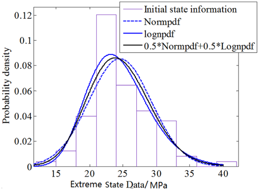
PDF curves fitted with the initial monitored extreme stress data.

Figure 6.

Initial state PDF and updated state PDF.

Dynamic nonlinear models based on the monitored data of the forward 83 days

Based on the forward 83 days’ monitored data and Figure 1, with equations (4)–(21) and (50), the built dynamic nonlinear models are as follows:

Observation equation

y_{t + 1} = θ_{t + 1} + ν_{t + 1}, ν_{t + 1} ~ N [0, V_{t + 1}], (t = 1, 2, \dots, T)

(51)

State equation

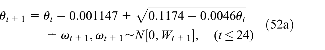
\begin{matrix} θ_{t + 1} = θ_{t} - 0.001147 + \sqrt{0.1174 - 0.0046 θ_{t}} \\ + ω_{t + 1}, ω_{t + 1} ~ N [0, W_{t + 1}], (t \leq 24) \end{matrix}

(52a)

and

\begin{matrix} θ_{t + 1} = θ_{t} - 0.001147 - \sqrt{0.1174 - 0.0046 θ_{t}} + ω_{t + 1}, \\ ω_{t + 1} ~ N [0, W_{t + 1}], (t > 24) \end{matrix}

(52b)

Initial state information

\begin{matrix} θ_{t} | D_{t} ~ 0.5 N [24.56, 4.6 7^{2}] + 0.5 LN [3.18, 0.1 9^{2}] \\ \approx 0.5 * N [24.56, 4.6 7^{2}] + 0.5 * N [23.17, 3.3 5^{2}] \end{matrix}

(53)

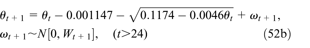
where y_t_+ 1 is the monitored extreme stress data at time t + 1, m_t_+ 1 is the state value of the monitored extreme stress at time t + 1, $ν_{t + 1}$ is observational error, and $ω_{t + 1}$ is state error, which means the uncertainty of state variable. V_t_+ 1 can be approximately obtained with the monitored stress data set D _t + 1, and $δ = 0.98, W_{t + 1} = - C_{t} + C_{t} / δ$ according to the actual engineering experience of the authors.^6,11,12 $LN [\cdot]$ is lognormal PDF, $C_{t}$ can be approximately obtained with equation (53).

With equations (51)–(53) and (34)–(49), based on the monitored extreme stress data from the 83rd day to the 89th day, the predicted extreme stress and prediction precision from the 84th to 90th day are, respectively, solved which are shown in Figures 7 and 8.

Figure 7.

Predicted and monitored extreme stress data.

Figure 8.

Prediction precision of dynamic nonlinear models based on MGPF algorithm.

From Figure 7, it can be noticed that the predicted data fit the changing rules of monitored extreme data; Figure 8 shows that the prediction precision of the built dynamic nonlinear models is nearly better and better with the updating of the monitored stress data. But there is a sudden increase between 87th and 88th day, and a decaying trend after 89th day. These two problems will be studied in the following papers by the authors.

Conclusion

This article first builds the dynamic nonlinear models based on the monitored data. Then, the MGPF algorithm is first given for structural stress information prediction. Finally, an actual example is provided to illustrate the feasibility and application of the proposed MGPF algorithm.

From the stress prediction results shown in Figure 7, the prediction value of the extreme stress fit the changing rules of the monitored value; the prediction precisions, shown in Figure 8, are both better and better with the updating of the monitored data, which shows that the proposed dynamic nonlinear models and given MGPF algorithm in this article are reasonable and feasible for structural extreme stress prediction. But there is a sudden increase between 87th and 88th day and a decaying trend after 89th day. These two problems will be studied in the following papers by the authors.

Footnotes

Acknowledgements

The authors would like to thank the editor and the anonymous reviewers for their constructive comments and valuable suggestions to improve the quality of the article.

Academic Editor: Yongming Liu

Declaration of conflicting interests

The author(s) declared no potential conflicts of interest with respect to the research, authorship, and/or publication of this article.

Funding

The author(s) disclosed receipt of the following financial support for the research, authorship, and/or publication of this article: This work was supported by the Fundamental Research Funds for the Central Universities (lzujbky-2015-300, lzujbky-2015-301).

References

Zou

YJ.

The role of structural health monitoring in bridge assessment and management. Thesis for the degree of Master of Science, Lehigh University, Bethlehem, PA, 2011.

Zhou

. A study on system integration technique of intelligent monitoring systems for soundness of long-span bridges. China Civ Eng J 2006; 39: 46–52 (in Chinese).

Miu

CQ.

Health monitoring system for the Runyang Yangtse River Bridge. J Southeast Univ 2003; 33: 544–548 (in Chinese).

Chana

THT

Yua

Tam

HY.

Fiber Bragg grating sensors for structural health monitoring of Tsing Ma bridge: background and experimental observation. Eng Struct 2006; 28: 648–659.

Dai

Zhang

Wang

Structural reliability assessment by local approximation of limit state functions using adaptive Markov chain simulation and support vector regression. Comput-Aided Civ Inf 2012; 27: 676–686.

Fan

DG.

Real-time reliability forecast of bridge structures based on multiple Bayesian dynamic linear models. J S China Univ Tech 2013; 41: 67–72 (in Chinese).

Guo

Bian

CD.

Condition assessment of long span bridges using Monte Carlo numerical simulation. J Highw Transp Res Dev 2005; 22: 26–30 (in Chinese).

SL.

Approaches of condition assessment and damage alarming of bridges based on structural health monitoring. Harbin, China: School of Civil Engineering, Harbin Institute of Technology, 2009 (in Chinese).

Wang

. Assessment of dynamic reliability of existing bridges having regard to time variations of target reliability indices. Bridge Construct 2007; supp 1: 132–134 (in Chinese).

10.

Fan

XP.

Bayesian forecasting of structural bending capacity of aging bridges based on dynamic linear model. In: Strauss

Frangopol

Bergmeister

(eds) Life-cycle and sustainability of civil infrastructure systems: proceedings of the 3rd international symposium on life-cycle civil engineering (IALCCE 2012), Vienna, 3–6 October 2012. London: Taylor & Francis, 2012, pp.268–274.

11.

Wang

Performance prediction and reliability management of concrete structures based on information updating. Beijing, China: School of Civil Engineering, Tsinghua University, 2006 (in Chinese).

12.

Wang

Liu

XL.

Evaluation and Bayesian dynamic prediction of deterioration of structural performance. Struct Infrastruct E 2010; 6: 663–674.

13.

Yang

YX.

Time-dependent reliability assessment and life prediction of concrete continuous beam bridge. Harbin, China: School of Civil Engineering, Harbin Institute of Technology, 2007 (in Chinese).

14.

Casas

JR.

Reliability-based assessment of masonry arch bridges. Constr Build Mater 2011; 25: 1621–1631.

15.

Catbas

Susoy

Frangopol

DM.

Structural health monitoring and reliability estimation: long span truss bridge application with environmental monitoring data. Eng Struct 2008; 30: 2347–2359.

16.

Frangopol

Strauss

Kim

Use of monitoring extreme data for the performance prediction of structures: general approach. Eng Struct 2008; 30: 3644–3653.

17.

Jing

ZL.

Particle filtering theory and its application. Beijing, China: Science Press, 2010.

18.

Peng

Liu

Miu

. Application of Gaussian mixture particle filter on state estimation. Danjian yu zhidao xuebao/J Proj Rocket Missile Guid 2007; 27: 271–274.

Dynamic extreme stress prediction of bridges based on nonlinear mixed Gaussian particle filtering algorithm and structural health monitoring data

Abstract

Keywords

Introduction

Dynamic nonlinear models based on SHM data

The quadratic function

The transformed approximate state equation based on quadratic function

The dynamic nonlinear model

Determination of the main probability parameters of dynamic nonlinear models

MGPF algorithm based on the nonlinear dynamic model

The approximate PDF (importance function) of p ( θ t + 1 | D t + 1 ) based on the extended Kalman filter

The MGPF algorithm based on the nonlinear dynamic model

Application to an existing bridge

Dynamic nonlinear models based on the monitored data of the forward 83 days

Conclusion

Footnotes

Acknowledgements

Declaration of conflicting interests

Funding

References

The approximate PDF (importance function) of $p (θ_{t + 1} | D_{t + 1})$ based on the extended Kalman filter