Modeling and performance analysis of a closed-loop supply chain using first-order hybrid Petri nets

Abstract

Green or closed-loop supply chain had been the focus of many manufacturers during the last decade. The application of closed-loop supply chain in today’s manufacturing is not only due to growing environmental concerns and the recognition of its benefits in reducing greenhouse gas emissions, energy consumption, and meeting a more strict environmental regulations but it also offers economic competitive advantages if appropriately managed. First-order hybrid Petri nets represent a powerful graphical and mathematical formalism to map and analyze the dynamics of complex systems such as closed-loop supply chain networks. This article aims at illustrating the use of first-order hybrid Petri nets to model a closed-loop supply chain network and evaluate its operational, financial, and environmental performance measures under different management policies. Actual data from auto manufacturer in the United States are used to validate network’s performance under both tactical and strategic decision-making, namely, (1) tactical decision—production policies: increase of recovered versus new components and (2) strategic decision—closed-loop supply chain network structure: manufacturer internal recovery process or recovery process done by a third-party collection and recovery center. The work presented in this article is an extension of the use of first-order hybrid Petri nets as a modeling and performance analysis tool from supply chain to closed-loop supply chain. The modularity property of first-order hybrid Petri nets has been used in the modeling process, and the simulation and analysis of the modeled network are done in MATLAB^® environment. The results of the experiments depict that first-order hybrid Petri nets are a powerful modeling and analysis formalism for closed-loop supply chain networks and can be further used as an efficient decision-making tool at both tactical and strategic levels. Unlike other researches on modeling supply chain networks that focus on evaluating individually cost, operational, or environmental aspects, the research here shows how first-order hybrid Petri nets can be extended to assess simultaneously operational, financial, and environmental network’s performance measures at different managerial decision-making levels. The results particularly are compelling for researchers and industrial practitioners who can use the same methodology in evaluating their network’s performance and making educated management decisions based on the performance results and the impact of their selected supply chain and manufacturing strategies.

Introduction

Preserving the current reserves of natural resources in the context of an increasing population, growing economies, rise in pollution, and increasing greenhouse gas emissions is vital for future generations. Therefore, sustainability issues have gained a huge interest among researchers, industrials, and policy makers in the last few decades. As the backbone of the world’s economy, manufacturing industries contributes by 30.7% to the world gross domestic product (GDP) and employs over 0.7 billion workforce worldwide. ¹ In the context of our research and the overall impact on the environment, manufacturing industries are one of the main sources of waste worldwide and their supply chain activities are a major consumer of energy and a significant source of greenhouse gas emissions. 35% of total greenhouse gas emissions are due to the use of heavy and light vehicles in the supply chain activities. ² For this reason and to better comply with government’s environmental regulations and sustainability policies, manufacturing industries are considering and adapting green supply chain (GSC) philosophy in their approach in both tactical and strategic managerial decision-making process. This green supply chain management (GSCM) philosophy provides the manufacturer with opportunities to achieve simultaneously more economical profit with limited resources and less environmental risks. Typically, a forward supply chain (FSC) can be viewed as a broad set of activities associated with the transformation of material, information, financial, and knowledge flows with the goal of satisfying end-user requirements with products and services from multiple interconnected entities (suppliers, manufacturers, transporters, distributors, etc.). ³ The opportunity seen by manufacturers is in the recovery process of products using end-of-life (EOL) strategies such as reuse, recycling, and remanufacturing. The retrieval of end products from customers for the purpose of recapturing value or proper disposal through the recovery process is called reverse supply chain (RSC). The possible interaction of forward and reverse flows requires a certain level of coordination, and therefore makes it mandatory for manufacturers to combine both flows within the same supply chain called green or closed-loop supply chain (CLSC). ⁴ Within the last decade, modeling and analysis of such complex systems for an effective decision-making within the GSC have attracted many researchers. Decision-making within a CLSC can be classified into strategic, tactical, and operational planning. Most researchers explored different decision-making levels with regard to operational and financial performance measures, ⁵ but very few have considered the environmental impact within a CLSC. Furthermore, a very few number of researchers considered integrating financial and environmental performance measurement in a CLSC and applied first-order hybrid Petri nets (FOHPN) analysis. Therefore, the aim of this research is to extend the use of FOHPN to CLSC networks modeling in different decision-making levels (tactical and strategic) and enable the simultaneous analysis of operational, financial, and environmental performance measures of the network. Indeed, following the presented methodology for simulation and analysis of the dynamic behavior of CLSC will assist industrial practitioners in evaluating operational, financial, and environmental aspects of their network’s performance and make educated decisions on that basis.

CLSC network’s modeling: a state-of-the art review

The main goal of this review is to identify the state-of-the-art in CLSC modeling research and what topics are considered as significant future research opportunities. ⁶ Between January 2007 and March 2013, a total of 382 papers are published in scientific journals. The gaps in modeling of CLSC networks are classified into the following: ⁶

• Nonlinear programming and convex optimization

• Queuing models ⁷

• Graph-based models (Petri nets)

• Markov decision process ⁸

• Piecewise interval programming ⁹

• Dynamic regression ¹⁰

• Statistical approaches ¹¹

• Interval mathematics ¹²

A limited number of Petri net models of supply chain are available in the literature, with very few Petri net models describing CLSC, especially using the FOHPN.

Viswanadham and Raghavan ¹³ proposed a dynamic modeling technique for analyzing FSC networks using generalized stochastic Petri nets (GSPNs). The customer order arrival process is assumed to be Poisson, and the processing at the facilities of the supply chain is considered as exponential. Their model considers both the procurement and delivery logistics of goods between any two members of the supply chain. They compared the supply chain network performance under the make-to-stock and the assemble-to-order management policies based on total cost which is the sum of inventory cost and delayed deliveries. The problem is formulated and then solved for decoupling point location problem in supply chains as a total relevant cost minimization. They also used the framework of integrated GSPN queuing network modeling by combining the use of GSPN for high level and a generalized queuing network at low level to solve the decoupling point location problem.

Mazzuto et al. ¹⁴ implemented a new methodology for designing a supply chain and evaluating the performance of all stakeholders involved in a production chain. The methodology was applied to a footwear supply chain using colored Petri nets (CPNs). The supply chain analyzed is a complex production system consisting of a network of manufacturers and material suppliers related to logistic systems responsible of transportation and storage. In the model, colored timed Petri nets represent a supply chain. Petri net places represent resources; tokens represent jobs, orders, or products; and colors represent job attributes. The main function of colors is to encode different data types and values specific to tokens. The structure of this network allows designers to easily conduct what-if analyses through multiple object-oriented simulations.

Dotoli et al. ¹⁵ proposed a model to describe material, financial, and information flows of a supply chain network at the operational level. The supply chain is described by a modular model based on FOHPN. Information flows are described in the proposed framework, and financial flows are presented by a discrete Petri net sub-model. The formalism can effectively describe supply chains by a linear discrete-time and time-varying state variable model that enables the designer to choose decision variables in the system. Different inventory controllers were modeled and tested to choose the one that leads to satisfactory throughput and inventory levels. The effectiveness and simplicity of the modeling technique was shown through the modeling and simulation of a case study under a standard management policy and with three different control strategies to evaluate its performance.

Haiyan ¹⁶ proposed a model of a RSC using GSPNs for RSC design in order to choose a more appropriate recovery mode. It identified two main recovery modes: (1) recycling or the remanufacturing is done by the original equipment manufacturer (OEM) and (2) outsourcing to a third party the recycling and remanufacturing activities. At first, the structure of a simplified RSC based on GSPN was built by identifying activity places, order places along with their capacities and connecting them properly by the identified transitions. Then, the coordinate Markov chain was developed, and the markings of the RSC are identified. Through analyzing Markov chain, the steady-state probability was solved. The approach provides some insights in modeling and simulation of RSC in order to choose the proper recycling mode. Therefore, two more detailed models of the two recycling modes have to be developed using GSPN, along with the calculation of the indicators such as the steady-state probability, timing of performance, changes in utilization, and efficiency of the whole system, so the model can be used by decision-makers to choose a favorable recycling mode. Table 1 summarizes the most relevant papers reviewed for modeling of FSC, RSC, and CLSC using different Petri nets for performance measurement purposes.

Table 1.

Literature review table (FSC/RSC/CLSC).

Research title	Scope	Author	Publication year
Performance analysis and design of supply chains: a Petri net approach	FSC	Viswanadham and Raghavan 13	2000
Supply chain modeling and managing, using colored Petri nets	FSC	Mazzuto et al. 14	2011
Hybrid Petri nets for modeling and performance evaluation of supply chains	FSC	Khilwani et al. 17	2010
Comparing management policies for supply chain via hybrid Petri net model	FSC	Dotoli et al. 18	2007
A first-order hybrid Petri net model for supply chain management	FSC	Dotoli et al. 15	2009
Modeling and analysis of reverse supply chain based on generalized stochastic Petri nets	RSC	Haiyan 16	2009
Modeling closed-loop supply chain system based on stochastic fuzzy Petri net	CLSC	Wang Jun-Yan 19	2013

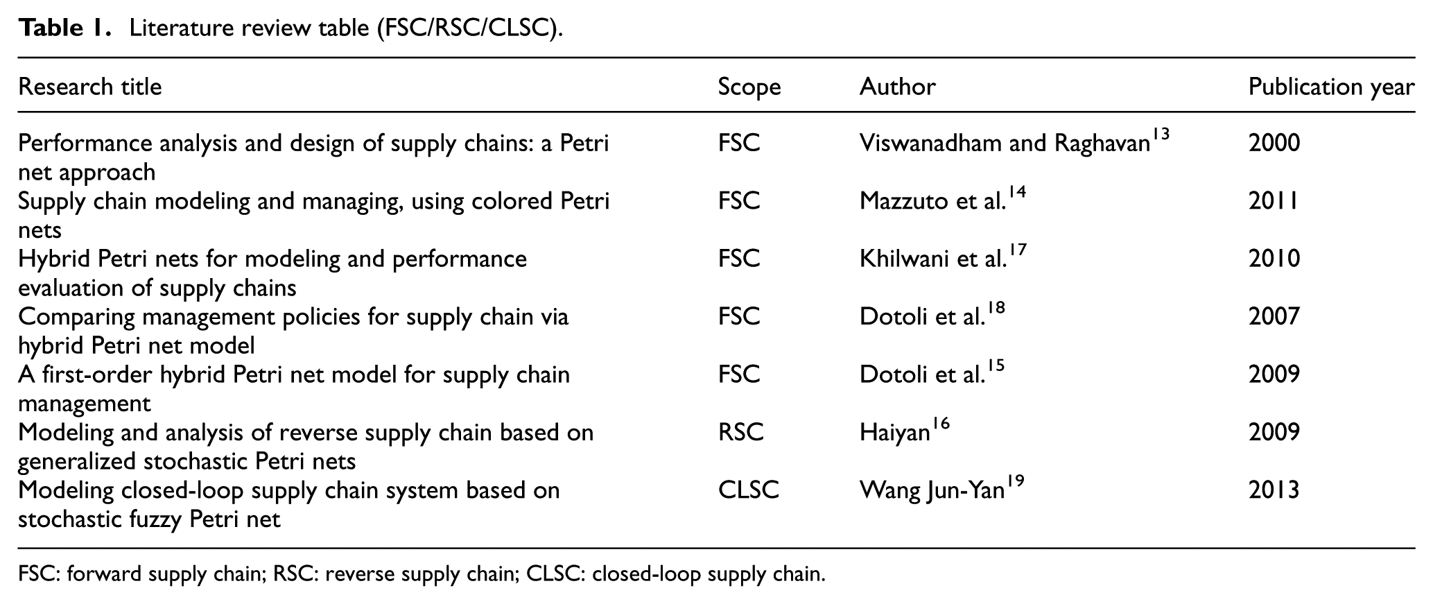
FSC: forward supply chain; RSC: reverse supply chain; CLSC: closed-loop supply chain.

Different extensions of Petri nets used for supply chain modeling

There are many extensions of Petri nets, and each of them has its unique properties to model a specific application.

In their review of Petri-net-based applications for supply chain management, invalid source specified pointed out the most frequently used Petri net extensions: ²⁰

GSPNs are widely used for modeling and analysis of real-time systems. GSPN includes two kinds of transitions: timed and immediate transitions. Timed transitions are modeled through an exponentially distributed random firing time while immediate transitions fire in zero time. ²⁰

Batch deterministic and stochastic Petri nets (BDSPNs) introduce batch components, new transition enabling and firing rules, and specific policies defining the timing concepts into the model. ²⁰

CPNs are developed for systems in which communication, synchronization, and resource sharing play an important role. Token types are specified through colors, where each color set determines the possible values of the tokens. ²⁰

High-level Petri net (HLPN) provides a simple graphical representation of hybrid systems and takes advantage of the modular structure of a Petri net in giving a compact description of systems composed of interacting subsystems, both time-continuous and discrete-event. The use of colors in the continuous places allows one to model continuous variables that may take negative values. ²⁰

FOHPN consists of continuous places holding fluid, discrete places containing a non-negative integer number of tokens, and transitions, either discrete or continuous. FOHPN was originally proposed in Balduzzi ²¹ and has been efficiently used in many application domains, such as manufacturing systems and inventory control. ¹⁸

The complex valued token Petri net, named jPN, facilitates the analysis of basic Petri nets while increasing the descriptive power. This extension of Petri nets is characterized by places containing two different types of tokens: real and imaginary tokens. The input functions, output functions, and initial marking can all take on complex numbers, which is the main difference between the jPN formulation and the basic Petri net. The complex structure of jPNs allows for the use of complex arithmetic and complex matrix algebra for their analysis. ²⁰

Trans-net is another variant of Petri net a variant of the Petri net. It is used to abstract and model the information, removing many of the complexities, while retaining the ability to analyze the more important characteristics of the supply chain. ²⁰

Advantages of using FOHPN formalism for CLSC modeling

The use of FOHPNs offers several significant advantages compared to the other Petri net models existing in the related literature: fluid approximation of flows reduces the dimension of the state space and therefore increases the computational efficiency of the model, the graphical feature allows for an easy modular modeling approach, and the mathematical aspects efficiently allow for the simulation of different scenarios and even a possible optimization of the system.

FOHPN theory

The FOHPN formalism was first presented by Balduzzi et al. ²¹ The formalism presented in this paper is based on the review of the above-mentioned paper along with the following two papers: Dotoli et al. ¹⁵ and Giua et al. ²²

Structure

A FOHPN is a bipartite-directed graph defined by the structure $\mathrm{PN}=(P,T,\mathrm{Pre},\mathrm{Post},\Delta ,F,\mathrm{RS})$ .

Place definition

Places represent possible states or conditions of the system. A place can represent data storage in information systems as it can represent buffers in manufacturing systems or any other storage locations. The set of places $P=P_d\cup P_c$ is partitioned into a set of discrete places $P_d$ (circles) and a set of continuous places $P_c$ (double circles). The cardinality of $P$ , $P_d$ , and $P_c$ is denoted as $n$ , $n_d$ , and $n_c$ , respectively.

Transition definition

Transitions describe events that may modify system states such as a process in a manufacturing system. The set of transitions $T=T_d\cup T_c$ is partitioned into a set of discrete transitions $T_d$ and a set of continuous transitions $T_c$ (double boxes). The set $T_d=T_I\cup T_D\cup T_S$ is further partitioned into a set of immediate transitions $T_I$ (bars), a set of deterministic timed transitions $T_D$ (black boxes), and a set of stochastic timed transitions $T_S$ (white boxes). The cardinality of $T$ , $T_d$ , and $T_c$ is denoted as $q$ , $q_d$ , and $q_C$ , respectively. We also denote the set of timed transitions as $T_t=T_S\cup T_D$ .

Firing function for discrete transitions: $\Delta$

A transition fires by moving its tokens from its input places and then deposits the tokens into each of its output places. The function $\Delta :T_D\to {\mathrm{ℝ}}^{+}$ specifies the timing associated to timed transitions. In particular, each transition $t_j\in T_D$ is associated to a constant firing delay ${\delta }_j=\Delta (t_j)$ . Additionally, in the case of timed stochastic transitions, $\Delta :T_S\to F$ assigns to each $t_j\in T_S$ a probability density function (pdf) that characterizes its firing delay (F is the set of probability density functions for a random variable that can only take non-negative values, as is the case with a firing delay). We associate to each $t_j\in T_S$ the average firing delay $\Delta (t_j)={\delta }_j=1/{\lambda }_j$ , where ${\lambda }_j$ is the average firing rate of the transition. In case the transition is exponential, ${\delta }_j$ represents the expected value of the associated distribution, while in case it is triangular, ${\delta }_j$ represents the modal value of such a distribution and we assume that the minimum and maximum values of the range in which the firing delay varies equal, respectively, $0.8{\delta }_j$ and $1.2{\delta }_j$ .

Firing function for continuous transitions: F

The function $F:T_C\to {\mathrm{ℝ}}_0^{+}\times {\mathrm{ℝ}}_{\infty }^{+}$ specifies the firing speeds associated with continuous transitions ( ${\mathrm{ℝ}}_{\infty }^{+}={\mathrm{ℝ}}^{+}\cup \{\infty \}$ ). For any continuous transition $t_j\in T_C$ , we let $C(t_j)=(V{\prime }_j,V_j)$ , with $V{\prime }_j<V_j$ . $V{\prime }_j$ represents the minimum firing speed (mfs) and $V_j$ represents the maximum firing speed (MFS).

Probability function for conflicting discrete transitions: random switch

A conflicting situation occurs when two transitions are both ready to fire but the firing of any leads to the disabling of the other transition (Figure 1).The function $\mathrm{RS}:T_d\to {\mathrm{ℝ}}^{+}$ associates a probability value called random switch to conflicting discrete transitions.

Figure 1.

Conflicting transitions.

Pre-incidence, post-incidence, and incidence matrices

The pre- and post-incidence functions that specify, respectively, the weight attached to the input arcs directed from places to transitions and the weights attached to the output arcs directed from transitions to places are ( ${\mathrm{ℝ}}_0^{+}={\mathrm{ℝ}}^{+}\cup \{0\}$ )

$$\mathrm{Pre}:P_c\times T\to {\mathrm{ℝ}}_0^{+},P_d\times T\to \mathbb{N}$$

$$\mathrm{Post}:P_c\times T\to {\mathrm{ℝ}}_0^{+},P_d\times T\to \mathbb{N}$$

We require (well-formed nets) that for all $t\in T_c$ and for all $p\in P_d$ , Pre(p, t) = Post(p, t). This ensures that the firing of continuous transitions does not change the marking of discrete places. The incidence matrix of the net is defined as $C(p,t)=\mathrm{Post}(p,t)-\mathrm{Pre}(p,t)$ . The restriction of C to $P_X$ and $T_Y(X,Y\mathrm{E}\{c,d\})$ is denoted as $C_{\mathrm{XY}}$ .

Marking function definition

A marking is a function that assigns to each discrete place a non-negative number of tokens, represented by black dots, and assigns to each continuous place a fluid volume. We partition the set of continuous places $P_C=P_0\cup P_{+}$ into a set of places $P_0$ (full dark circles) whose marking is always equal to 0, and a set of places $P_{+}$ (double circles) whose marking may assume any non-negative real number. Therefore, $m:P_{+}\to {\mathrm{ℝ}}_0^{+},P_0\to 0,P_d\to \mathbb{N}$ . The marking of place $p_i$ is denoted as $m_i$ , while the value of the marking at time τ is denoted as m(τ). The restriction of m to $P_d$ and $P_c$ is denoted with $m^d$ and $m^c$ , respectively. A FOHPN system $〈N,m({\tau }_0)〉$ is a FOHPN N with an initial marking $m({\tau }_0)$ .

Enabling and firing

Firing rule for discrete transitions

The enabling of a discrete transition depends on the marking of all its input places, both discrete and continuous. A discrete transition t is enabled at m if for all $p_i\in •t,m_i\ge \mathrm{Pre}(p_i,t)$ , where $•t$ denotes the preset of transition t, $•t=\{p\in P,\mathrm{Pre}(p,t)>0\}$ .

Firing rule for continuous transitions

A continuous transition is enabled only by the marking of its input discrete places. The marking of its input continuous places, however, is used to distinguish between strongly and weakly enabling. A continuous transition $t_j$ is enabled at time $\tau$ if and only if all its input discrete places $p^k\in P^d$ have $m_k(\tau )\ge \mathrm{Pre}(p_k,t_j)$ , and all its input continuous places $p_i\in P_C$ satisfy the following condition: either $m_i(\tau )>0$ or $p_i$ is fed. $t_j$ is strongly enabled if all input continuous places of $t_j$ have a not-null marking, else $t_j$ is weakly enabled. In addition, the enabling state of a continuous transition continuous transition $t_j$ defines its admissible IFS denoted by ${\nu }_j$ .

Definition (admissible IFS vectors): let $〈N,m〉$ be an FOHPN system with $n_c$ continuous transitions and incidence matrix C. Let $T_{\epsilon }(m)\subset T_C(T_N(m)\subset T_C)$ be the subset of continuous transitions enabled (not enabled) at m, and $P_{\epsilon }(m)=\{p\in P_{+}\setminus m_P=0\}$ be the subset of empty continuous places in $P_{+}$ . Any admissible IFS vector $\nu =[{\nu }_1,\dots ,{\nu }_{n_c}{]}^T$ at m is a feasible solution of the following linear set

$$\begin{array}{l}{V}_j-{\nu }_j\ge 0\forall t_j\in T_{\epsilon }\left(m\right)\\ {\nu }_j-{V^{\prime }}_j\ge 0\forall t_j\in T_{\epsilon }\left(m\right)\\ {\nu }_j=0\forall t_j\in T_N\left(m\right)\\ \sum _{t_j\in T_{\epsilon }}C(p,t_j)·{\nu }_j\ge \forall p\in P_{\epsilon }\left(m\right)\\ {\displaystyle \sum _{t_j\in T}C(p,t_j)·{\nu }_j=0}\forall p\in P_0\end{array}$$

where ${\mathrm{V}}_{\mathrm{j}}$ and ${\mathrm{V}}_{\prime }^{\mathrm{j}}$ are, respectively, the MFS and mfs of continuous transition ${\mathrm{t}}_{\mathrm{j}}$ . The set of all feasible solutions is denoted as $\mathrm{S}(\mathrm{N},\mathrm{m})$ .

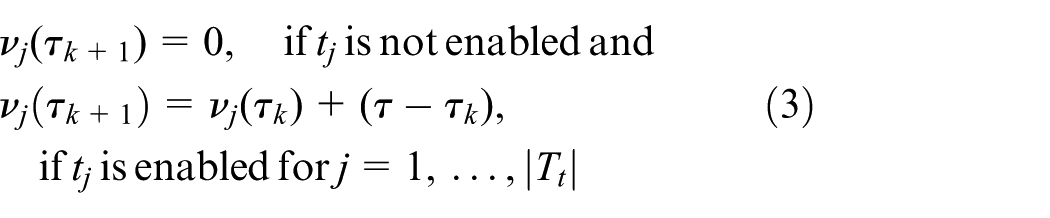
Net dynamics

We denote in hybrid models two behavioral levels lower and higher, respectively, related to time-driven and event-driven dynamics.

At the lower level

The continuous evolution of the net is described by first-order fluid models in which the continuous flows have constant rates and the fluid content of each continuous place varies linearly with time. The occurrence of time-driven macro-events is characterized by the following: (1) a discrete transition fires and leads to changing the discrete marking and enabling/disabling a continuous transition and (2) a continuous place becomes empty and leads to changing the enabling state of a continuous transition from strong to weak.

We can write the equation that describes the evolution in time of the marking of a place $p_i\in P_C$ as $m_i(\tau )=\sum _{t_j\in T_C}C(p_i,t_j)\times {\nu }_j(\tau )$ . We denote by $\nu (\tau )=[{\nu }_1(\tau ),\dots ,{\nu }_{n_c}(\tau ){]}^T$ the IFS vector at time τ.

Let ${\tau }_k$ and ${\tau }_{k+1}$ be the occurrence times of two consecutive macro-events; we assume that within the interval of time $[{\tau }_k,{\tau }_{k+1}]$ , denoted as a macro-period, the IFS vector is constant and we denote it as $\nu ({\tau }_k)$ . Then, the continuous behavior of a FOHPN for $[{\tau }_k,{\tau }_{k+1}]$ is described as

$$\{\begin{array}{c}\hfill m^c(\tau )=m^c({\tau }_k)+C_{\mathrm{cc}}\nu ({\tau }_k)(\tau -{\tau }_k)\hfill \\ \multicolumn{1}{c}{m^d(\tau )=m^d\left({\tau }_k\right)}\end{array}$$

(1)

At the higher level

A discrete-event model describes the macro-behavior of the net due to event-driven dynamics. In this case, we consider the following two types of macro-events: (1) a continuous place, whose marking is increasing, reaches a flow level that enables a set of discrete transitions and (2) a continuous place, whose marking is decreasing, reaches a flow level that disables a set of discrete transitions.

The evolution of the net at the firing of a discrete transition $t_j\in T_d$ at $m({\tau }_k^{-})$ yields the following marking

$$\{\begin{array}{c}\hfill m^c({\tau }_k)=m^c({\tau }_k^{-})+C_{\mathrm{cd}}\sigma ({\tau }_k)\hfill \\ \multicolumn{1}{c}{m^d({\tau }_k)=m^d({\tau }_k^{-})+C_{\mathrm{dd}}\sigma ({\tau }_k)}\end{array}$$

(2)

where $\sigma ({\tau }_k)$ is the firing count vector associated to the firing of transition $t_j$ at time ${\tau }_k$ . To each timed transition $t_j\in T_d$ , a timer ${\nu }_j$ is associated.

The timer evolution within the macro-period $[{\tau }_k,{\tau }_{k+1}]$ for each transition $t_j\in T_d$ is

$$\begin{array}{cc}\multicolumn{1}{c}{}& {\nu }_j({\tau }_{k+1})=0,\mathrm{if}{t}_j\mathrm{is\; not\; enabled\; and}\hfill \\ \multicolumn{1}{c}{}& {\nu }_j\left({\tau }_{k+1}\right)={\nu }_j({\tau }_k)+(\tau -{\tau }_k),\hfill \\ \multicolumn{1}{c}{\mathrm{if}{t}_j\mathrm{is\; enabled\; for}j=1,\dots ,\left|T_t\right|}\end{array}$$

(3)

The timer of $t_j$ is reset to 0 if it is disabled or it fires.

A FOHPN system can be described in the macro-period $[{\tau }_k,{\tau }_{k+1}]$ by the discrete-time state equation as

$$x\left({\tau }_{k+1}\right)=A\left({\tau }_k\right)x\left({\tau }_k\right)+B\left({\tau }_k\right)u\left({\tau }_k\right)$$

(4)

The behavior of the system is described in the macro-period $[{\tau }_k,{\tau }_{k+1})$ by the following equation

$$\left[\begin{array}{c}{m}^c\left({\tau }_{k+1}\right)\\ m^d\left({\tau }_{k+1}\right)\\ \nu \left({\tau }_{k+1}\right)\end{array}\right]=\left[\begin{array}{ccc}I& 0& 0\\ 0& I& 0\\ 0& 0& D\left({\tau }_k\right)\end{array}\right]\ast \left[\begin{array}{c}{m}^c\left({\tau }_k\right)\\ m^d\left({\tau }_k\right)\\ \nu \left({\tau }_k\right)\end{array}\right]+\left[\begin{array}{cc}{C}_{cc}\nu \left({\tau }_k\right)& C_{dc}\\ 0& C_{dd}\sigma \left({\tau }_k\right)\\ f\left({\tau }_k\right)& 0\end{array}\right]\ast \left[\begin{array}{c}{\tau }_{k+1}-{\tau }_k\\ \sigma \left({\tau }_{k+1}\right)\end{array}\right]$$

(5)

The net state is given by the net marking and by the vector $\nu ({\tau }_k)$ of timers associated to discrete timed transitions at time ${\tau }_k$ . The net input includes the macro-period duration $[{\tau }_{k+1}-{\tau }_k)$ and the firing vector $\sigma ({\tau }_{k+1})$ associated to the firing of transition t_j at ${\tau }_k$ . The elements of matrix $D({\tau }_k)$ and vector $f({\tau }_k)$ are equal to 0/1 and depend on the macro-event occurring at the sampling instant.

Research significance

CLSC or GSC consists of a series of complex and integrated system of networks that require the use of advanced mathematical modeling and analysis tools for accurate design, performance analysis, and the measurement of their efficiency. Petri nets are considered as an ideal graphical modeling technique due to its strong mathematical foundation and a well-developed theory that can be used for the design and analysis of complex systems. Petri nets are able to model systems with event’s precedence, concurrency, and synchronization. FOHPNs are an extension of hybrid Petri nets that use fluid approximation of flows to reduce the dimension of the state space which increases the computational efficiency of the models. ¹⁵ FOHPNs are an effective tool to model and analyze the performance of complex systems such as green supply chain networks (GSCNs). The analysis results will assist industrial practitioners in making educated and practical decisions for an optimal management of GSCN.^15,21,22 Decision-making within CLSC is made at three major levels of operations. These are strategic, tactical, and operational. The strategic planning or design of a CLSC is a long-range planning that involves the structuring of the supply chain over the next several years. ²³ For example, strategic decisions impact issues such as the selection of used products, the evaluation of collection centers, the evaluation of recovery facilities, and the optimization of transportation of goods. ²³ Tactical or midterm planning in a CLSC is usually addressed in conjunction with strategic planning. The critical decision variable at this stage includes the quantities of flows between supply chain network entities. ⁶ Operational or short-term planning in a CLSC aims at determining the best possible manner of how to handle incoming customer orders as in a typical FSC in addition to CLSC-related issues such as disassembly, and recovery planning and scheduling. ²³ We analyzed a CLSC case study under tactical and strategic decision-making levels. This is to demonstrate the effectiveness of FOHPN models for GSCN and to illustrate how to measure operational, financial, and environmental performances within different decision-making contexts. For both tactical and strategic levels, same methodology is applied. Once the network structure and the key performance parameters are defined, the network is further decomposed into subsystems of supplier, manufacturer, transporter, and so on. Each subsystem is modeled individually, and then all elementary modules are merged using transportation transitions to form the final network model. ²⁴ After implementing the graphical model combined with the required input data (firing speeds for continuous transitions, average firing delay for discrete transitions, parameters of inventory policy adopted, capacities for continuous places, and initial markings) into a MATLAB environment, an additional constraint, namely, the choice of IFS for each macro-period is developed and the simulation results are analyzed for each scenario. In our initial analysis, flow maximization constraints of all flow rates are selected. This constraint allows for the maximization of the selected performance index $J=1^T·v$ , where ν represents the vector of firing speeds of all continuous transitions. Finally, the performance measures are computed and used to draw conclusions about the most feasible management decisions to implement. An open-source graphical hybrid Petri net editor (Snoopy2) is used to edit the FOHPN model ²⁵ and network simulation used an open-source software (Hyphens). This tool is a MATLAB toolbox for simulation and analysis of FOHPN. ²⁶

GSC/CLSC network under different tactical management strategies

The case study represents a CLSC network of a US auto manufacturer. For simplification purposes, the presented network is restricted to the assembly of front and rear axles to the cars in process. It includes a number of interconnected entities such as suppliers, original car manufacturer, car dealers, transporters, and a third-party collection and recovery center (Figure 2).

Figure 2.

CLSC network description.

Front and rear axles are, respectively, provided by suppliers 1 and 2 to the manufacturer where they are assembled to cars in process. Car dealers’ requests for cars are satisfied by the car manufacturer through transporters. The car dealers fulfill customers’ stochastic demand. Some used cars are returned by customers to the collection and recovery center where cars are disassembled and used axles recovered. The model includes both material and information flows within the CLSC network. Three scenarios based on three different production planning decisions are investigated to evaluate the operational impact of each on the network performance. In the first scenario, the original manufacturer receives 80% of its supplies from suppliers of new axles, and the remaining 20% from the recovery center. In the second scenario, the original manufacturer receives 20% of its supplies from suppliers of new axles, and the remaining 80% from the recovery center. In the final scenario, the original manufacturer uses 50% of its supplies from suppliers of new axles, and 50% from the collection and recovery center. Performance measures selected are (1) average car throughput, (2) average manufacturer inventory level, and (3) average lead time. Return rates of used cars and returned axles quality due to different usage patterns are noted as µ1 є [0, 1] and µ2 є [0, 1] and are, respectively, assumed to be 80% and 70%. Additionally, we assumed that the described CLSC is managed based on a push policy and that input buffers are managed based on a (Q, R) inventory policy. A push-type system can be described as a top-down planning system because all production quantity decisions are derived from forecasted demand and the system produces as many products as previously forecasted. ²⁷ A (Qs, R) inventory policy is a fixed replenishment quantity inventory policy. When the inventory level on-hand falls below a certain replenishment point, R, a replenishment order for a certain quantity, Q, namely, order quantity, is generated.

Modules of elementary entities

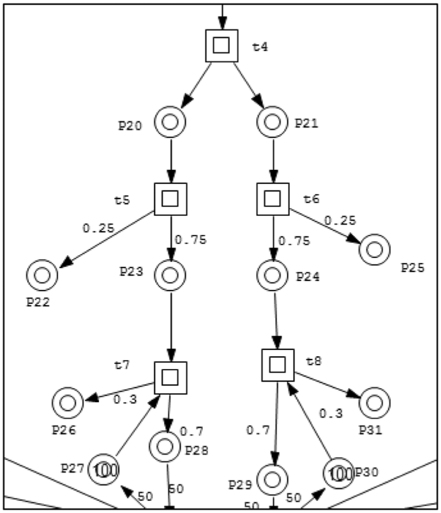
The supplier module (Figure 3) is defined by continuous transition t1 that represents the order processing of axles, continuous place P1 that represents axles output buffer of capacity C = 5000 and continuous place P2 corresponding to free output buffer space. We assumed the manufacturer is adopting Q = 50 and R = 20 inventory policy for component supply which is illustrated using arc weights (Q = 50) between stochastic transportation transition t9 and places P1 and P2. Transporter (Figure 4) is modeled based on two discrete transitions: (1) stochastic transition t9 for the transportation operation, assumed as a triangular distribution with parameters (0.8, 1, 1.2) h, and (2) discrete instantaneous transition t11 random switch that specifies the probability that the original manufacturer chooses to get supplies from suppliers of new axles. The manufacturer module shown in Figure 5 uses (1) continuous places P6 and P5 (input buffer and complementary space of front axles), (2) continuous places P8 and P7 (input buffer and complementary space of rear axles), (3) continuous places P10 and P9 (output buffer and complementary space of assembled cars), and (4) continuous transition t3 as assembly operation. The car dealer module (Figure 6) is based on (1) continuous places P11 and P12 (input buffer and complementary space to describe the Q = 30 and R = 10 policy adopted), (2) stochastic transition t15 (customer’s car request) assumed exponential, (3) continuous place P15 (collects the cars obtained by the car dealer and sold to customers), and (4) stochastic transition t17 to represent the return of used products. The arc weights between (P12–t15) and (t15–P12) represent the stochastic demand for cars. Finally, we assumed that the used products are sorted, cleaned, and tested (Figure 7) by the recovery center and introduced in the original manufacturing process of manufacturer. The process is modeled using continuous places representing the work in process buffers and continuous transitions to model the recovery, namely, disassembly, sorting, cleaning, and testing activities. Figure 8 illustrates the sub-model for the collection and recovery center. The firing speeds for continuous transitions and the average firing delays for discrete ones are illustrated in Table 2, and the CLSC network used for tactical decision-making is shown in Figure 9.

Figure 3.

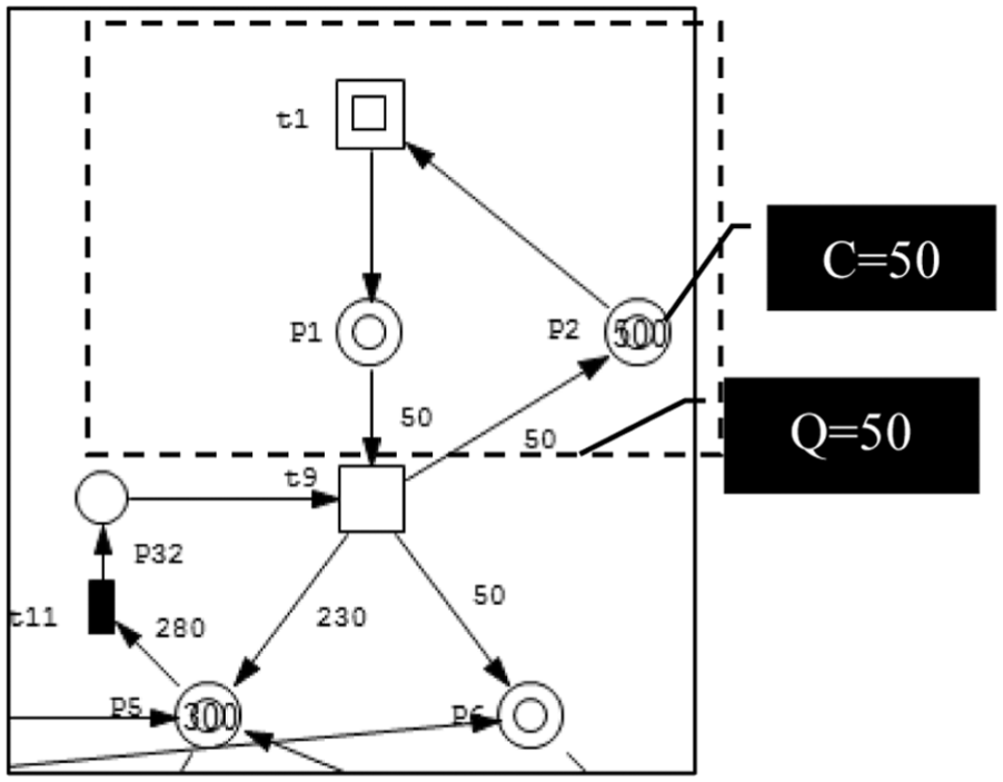
Supplier sub-model.

Figure 4.

Transporter sub-model.

Figure 5.

Manufacturer sub-model.

Figure 6.

Car dealer sub-model.

Figure 7.

Recovery of axles.

Figure 8.

Collection and recovery center sub-model.

Table 2.

Firing speed (average firing delay) of continuous (discrete) transitions for final CLSC.

Continuous transitions		Discrete transitions
	[Vmin, Vmax]	Exponential	Average firing delay (h)	Immediate	Average firing delay (h)	Triangular	Average firing delay (h)
t1, t2, t4	[0,10]	t15, t16, t17, t18	1	t11, t12, t21, t22	0	t9, t10, t13, t14, t19, t20	1
t3	[0,8]
t5, t6, t7, t8	[0,20]

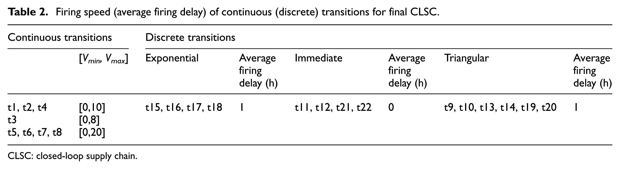
CLSC: closed-loop supply chain.

Figure 9.

Final CLSC network model.

Performance analysis

Selected performance measures for analysis and decision-making include the following:

• The average manufacturer throughput, TH, defined as the average number of cars assembled by the manufacturer in a time unit. It is represented in the model by the average firing speed of transition t3 in a simulation period;

• The average input inventory in manufacturer during the run time: the sum of the amount of axle’s storage in manufacturer input buffers during the run time. It is represented in the model by the average markings of places P6 and P9;

• The average output inventory in manufacturer during the run time: the sum of the amount of cars storage in manufacturer output buffer during the run time, represented by the average marking of place P10;

• The average manufacturer inventory I, that is, the sum of the amount of storage in all buffers during the run time;

• The lead time, LT = I/TH, is a measure of the time spent by the manufacturer to assemble a car.

The simulation results for the three scenarios are summarized in Table 3. The results are based on 20 replications using 500 h of operations with a transient period of 100 h and considering a 95% confidence interval.

Table 3.

Simulation results based on mixed product percentages.

Parameter	80% 20%	50% 50%	20%80%
TH	6.62 units/h	1.6 units/h	1.1 units/h
I	51 units	41.47 units	13 units
LT	7.70 h	26 h	11.82 h

GSC/CLSC network under different strategic management strategies

The primary goal of simulating two scenarios under different CLSC structures is to evaluate the operational, financial, and environmental implications of investing in EOL strategies. The first scenario is that the recovery process of axles is done by an external recovery center and supplies the original manufacturer with rebuilt axles. The second scenario is that the original manufacturer has incorporated a recovery process for used axles into its original production system. The critical performance measures of these two scenarios are the net profit of the manufacturer and the CO₂ emission cost related to transportation activities within the GSCN. The objective is to identify clearly the scenario that maximizes profit margins and minimizes CO₂ emissions/cost of CO₂ emissions. The calculation of greenhouse gas emissions, especially CO₂ generated by a certain mode of transportation is a nonlinear function including a number of major factors such as load, speed, and coefficient of drag as reported by EPA report. ²⁸

Since the scope is for strategic decision-making, we plan to use estimates of emissions. Therefore, we assume a unit transportation cost of 8.42 cents per ton-mile and unit emission cost of 0.86 cents per ton-mile for a general freight truck. ²⁹ First scenario: in addition to the tactical FOHPN model, a discrete Petri net part was developed and integrated into the overall model to represent the financial flows. Discrete places are then used to track the number of transportation operations. Also, the funds availability for each entity is represented by a set of discrete places, and stochastic transitions were used to represent the exchange of money between the network entities. Figure 10 shows the modeling of financial flow between supplier and the original manufacturer using discrete places P37 and P40 to refer as the available funds for the supplier and the manufacturer, respectively. Discrete place P36 (represents the occurrence of a transportation operation) is incremented by one token whenever a transportation operation occurs (firing of t10) which results in firing transition t24 to initiate fund transfer from manufacturer (P40) to supplier (P37). The transfer amount from manufacturer to supplier is calculated as follows: (Price of ordered axles + Cost of order transportation noted TrC)

$$\begin{array}{cc}\multicolumn{1}{c}{}& \mathrm{Price\; of\; ordered\; axles}=\mathrm{unit}\frac{\mathrm{price}}{\mathrm{axle}}*\mathrm{order\; quantity}\hfill \\ \multicolumn{1}{c}{}& \mathrm{Price\; of\; ordered\; axles}=\frac{300\$}{\mathrm{unit}}*50\mathrm{units}=15,000\$\hfill \\ \multicolumn{1}{c}{}& \mathrm{TrC}=\mathrm{unit\; transportation\; cost}*\hfill \\ \multicolumn{1}{c}{}& \mathrm{truck\; weight}*\mathrm{distance\; between\; supplier}\hfill \\ \multicolumn{1}{c}{}& \mathrm{and\; manufacturer}\hfill \\ \multicolumn{1}{c}{}& \mathrm{TrC}=8.42\frac{\mathrm{cents}}{\mathrm{ton}*\mathrm{mile}}*3\mathrm{tons}*500\mathrm{miles}=\$126.3\hfill \end{array}$$

Figure 10.

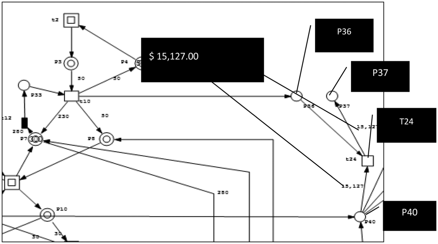
Modeling of financial flow between supplier and manufacturer.

Therefore, the amount transferred is equal to 15,000.00 + 126.3 = $15,127.00 and the weight of arcs (t24–P37) and (P40–t24) is $15,127.00 as shown in Figure 10.

Financial transfer amounts were calculated similarly between the remaining entities in the network. Figure 11 illustrates the final model describing material, financial, and information flows for the first scenario. The following assumptions are used for the analysis of case study although these parameters can be updated based on the case under consideration:

• Each entity (supplier, manufacturer, and third party) has a transporter module linked to it and offers paid transportation services to its clients;

• A car produced using returned axles has the same quality as a car produced using a new axle;

• Producing a car using reused axles is less costly than using new ones. In other words, the savings are greater than the cost of the recovery process (disassembly, inspection, etc.);

• The return and quality rates of axles are, respectively, equal to 80% and 70%;

• Total cost = CI (cost of inputs from suppliers or recovery center + transportation service cost paid to suppliers or third-party recovery center) + PRC (production cost estimated at 50% of the revenue);

• Manufacturer net profit = revenue (sold cars + transportation service to car dealers) − total cost;

• Price of a new axle = 300 $/unit, price of a used axle = 200 $/unit, price of a new car = 50,000 $/unit, price of a returned car = 10,000 $/unit;

• Transportation unit cost is 8.42 cents/ton-mile and unit emission cost is 0.86 cents/ton-mile;

• Distances: (supplier–manufacturer = 500 miles, manufacturer–dealer = 200 miles, dealer–recovery center = 200 miles, recovery center–manufacturer = 700 miles).

• (80% new axles, 20% reused axles) product mix;

• All stochastic transitions representing financial transfer have an exponential distribution with an average delay of 1 h.

The performance measures of interest are the average manufacturer throughput, CO₂ emission cost related to transportation activities, and manufacturer net profit.

Figure 11.

Final CLSC network model (strategic decision-making).

Scenario 1 experimental results

As calculated in the previous section, the average manufacturer TH is 6.62 units/h.

The CO₂ emission cost is calculated as the product of the unit emission cost, truck weight, distance between entities, and the number of transportation operations (number of times a transportation transition fires). It corresponds to a value of US$5250. For the auto manufacture case, net profit is the difference between the final and initial markings of discrete place P(40) for the simulation run. It corresponds to a value of US$2,715,000.

The second scenario in strategic decision-making assumes that recovery process of axles is done internally by the manufacturer. Therefore, the adaptation of the previous model to the context of the second scenario requires the following modifications:

• The cost of a reused axle recovered internally is 100 $/unit compared to 200 $/unit if recovered by a third-party collection and recovery center;

• The material handling time from the internal recovery process to the assembly line is negligible (convert stochastic transitions t19 and t20 to instantaneous transitions);

• The setup cost of the infrastructure for the recovery process is assumed to be included in the estimation of the production costs.

The experimental results of scenario 2 show that the average throughput is 7 units/h, the CO₂ emission cost related to transportation activities is US$4750, and a manufacturer net profit of US$3,335,000.

Conclusion

This article focuses on modeling and analysis of CLSC performance at different management levels (tactical and strategic). FOHPN formalism, an extension of Petri nets that uses the fluid approximation to reduce the state space dimension required for the simulation, maps the dynamics of the CLSC. Actual data from auto manufacturer in the United States are used to validate network’s performance under both tactical and strategic decision-making. The proposed FOHPN models describe material, information, and financial flows and allows for the simultaneous analysis of operational (average throughput, average inventory levels, and lead time), financial (total cost and transportation cost), and environmental (CO₂ emission cost) performance measures. Therefore, the obtained experimental results can provide practitioners with real-time assistance through their decision-making process.