Sage Journals: Discover world-class research

Abstract

The flow field of molten iron in the desulfurization process utilizing the mechanical stirring method under three different conditions was investigated using numerical simulation. The three conditions were central and eccentric stirring with the standard impeller and central stirring with the worn impeller, respectively. Three 1/20-scale numerical models were established and four inspection regions were set up on them. In all, 600 sets of instantaneous velocity fields for each model were exported and proper orthogonal decomposition technique was applied to deal with the data. The macroscopic flow field in the normal model operating under standard conditions was analyzed, which found that the mean flow has a relatively large fluctuation in flow field despite having a high proportion in total kinetic energy. A steady close relationship was revealed between the first two modes by studying the correlation of their coefficients. The first four modes were comparatively analyzed, which reflected that the change in the mean flow in the ladle using a worn impeller is slow and eccentric stirring is beneficial to desulfurization due to the asymmetry of the flow field on two sides.

Keywords

Mechanical stirring flow field proper orthogonal decomposition desulfurization stirred tank

Introduction

Mechanical stirring method was widely applied to the molten iron desulfurization process in the steelmaking process due to its efficiency and low operation cost; the crucial operation is to insert a vertical blade impeller into molten iron and then to stir, while flux is added on the liquid level.^1,2 Molten iron which is the primary phase in the process of desulfurization is in the state of motion all the time, and its flow pattern is critical to ensure the high quality of desulfurization.

The ladle for desulfurization is a kind of unbaffled stirred tank, which receives great attention as it has advantages in the industries of food, bio-engineering, and chemicals.^3,4 Although there exists low utilization of power and it cannot give rise to strong mix with respect to the baffle tanks, some researches also focus on the flow of the unbaffled stirred tank. Yang and Zhou⁵ studied the effect of gravity on pressure and velocity distributions. Montante et al.⁶ investigated the different effect between coaxial and eccentric agitation. Galletti et al.⁷ paid attention to the effect of geometrical parameters such as eccentricity and impeller blade thickness on the flow motion. Hidalgo-Millan et al.⁸ investigated the effect of the shaft eccentricity on the pumping capacity. The main feature of unbaffled stirred tanks is the strongly swirling liquid motion, which due to centrifugal effects leads to the formation of a whirlpool in the tank, and its shape mainly depends on the whole flow field as a result of centrifugal forces acting on the rotating liquid. Smit and Düring⁹ pointed out that liquid tangential velocity mainly depends on the distance from the shaft and the axial variation is small except at the bottom of the tank. Lamarque et al.¹⁰ dealt with the large-eddy simulation (LES) of a complex turbulent free surface flow in an unbaffled mixing tank reactor; they pointed out that coherent structures may have a strong impact on mixing in the reactor. Busciglio et al.¹¹ investigated the shape of the free surface with different impeller geometries by digital image analysis coupled with a suitable shadowgraphy-based technique.

Advanced techniques that generate a huge number of data such as particle image velocimetry (PIV) and numerical simulation are available nowadays, in terms of instantaneous velocity fields, so advanced data processing methods are required to extract useful information from the source data. Proper orthogonal decomposition (POD) is an excellent tool that can find the optimal representation of the field realizations from data sequence. The POD technique was first introduced in the context of turbulence by Lumley¹² to identify coherent structures in turbulent flows. In order to reduce the computational effort involved in solving the eigenvalue problem, the snapshot POD method¹³ is proposed, and snapshot POD studies were reviewed by Tabib and Joshi¹⁴ in the field of chemical engineering. In two-dimensional (2D) problem, each eigenvalue represents the flow kinetic energy contributed by its corresponding POD mode, and the combination of several POD modes with large eigenvalues can basically reflect the prominent main flow. Many researchers have used POD technique to analyze flow field since it appeared. The hydrodynamics in stirred vessel was studied using POD by Moreau and Liné,¹⁵ Gabelle et al.,¹⁶ and Liné et al.;¹⁷ meanwhile, POD technique was also applied to other applications such as three-dimensional (3D) large-scale structures for drag-reducing flow,¹⁸ the studies of characteristics of wake behind a cylinder,^19,20 and the interactions between the underlying turbulent features in corrugated channel flows.²¹

The spread of flux and the diffusion of sulfide ions in molten iron have great influence on the desulfurization efficiency in the process of desulfurization, and there is a close relation between the flow field in the ladle and them, hence it makes sense to study the flow field in the ladle with mechanical stirring. In this article, the information of flow field in three scaled-down models with different conditions was extracted by POD technique from a series of transient data that were obtained by numerical simulation and then the characteristics of POD modes were analyzed and compared.

Numerical simulation arrangement

Simulation model

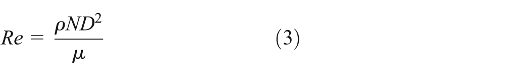
The free surface and the motion of molten iron in the ladle both have strong influence on the entire flow field in the desulfurization process; therefore, on the basis of meeting the requirements of Froude criterion, the Reynolds number of simulation models in this article entered the second self-modeling region, which brought simulation models closer to the real system. The forces acting on molten iron include inertia force, shear force caused by the viscous effect, and the gravity that pull liquid back to a stationary status; there exists the following equation while the model satisfies the Froude criterion

Fr = {(\frac{d V^{2}}{g})}_{m} = {(\frac{d V^{2}}{g})}_{p}

(1)

where d is the diameter of the impeller, V is the rotation speed of the impeller, g is the gravitational acceleration, the subscript m indicates the models, and the subscript p indicates the real system. The rotation speed in models can be formulated by equal Froude number

V_{m} = V_{p} {(\frac{d_{p}}{d_{m}})}^{\frac{1}{2}}

(2)

The parameters of the real system are shown in Table 1.

Table 1.

The parameters of real system.

Scheme	Parameter	Value
Structure	Tank diameter (m)	2.6
	Tank height (m)	3
	Number of blades	4
	Blade height (m)	0.7
	Blade top diameter (m)	1.15
	Blade bottom diameter (m)	1.05
	Blade thickness (m)	0.325
Operating	The rotation speed of impeller (r/min)	90
Molten iron	Dynamic viscosity (Pa s, 1300°C)	0.0384
Molten iron	Density (kg/m³)	7140

The proportion between the models and real is 1:20. The rotation speed of the impeller obtained from equation (2) is set to 402.5 r/min. According to turbulence theory, the turbulence features in scaled-down model are similar to that in the real system as Reynolds number up to the second self-modeling region. By the calculation formula of Reynolds number

Re = \frac{ρ N D^{2}}{μ}

(3)

It is known that the density or dynamic viscosity can be chosen to adjust Reynolds number. The inertia of molten iron will vary if the density is changed, so we choose changing dynamic viscosity.

On the actual desulfurization stirring, the wear of the blades of the impeller increased with the growing usage times; therefore, the chamfered blade in models was picked to represent the worn blade. The rotation speed needed to increase gradually to gain similar hydrodynamic conditions in actual practice with the worn blades. Accordingly, it was set to 450 r/min in model that owns worn blades.

The ladle vehicle cannot stay at the same position each time for the impact of inertia and friction, which caused the impeller to often deviate from the ladle center. To analyze this case, a model having eccentricity between the impeller and the ladle was built in the numerical simulation.

Three models were included in this article: the normal model, the eccentric model, and the worn model, which represented the model utilizing central and eccentric stirring with the standard impeller and central stirring with the worn impeller, respectively. The parameters of three models are shown in Table 2.

Table 2.

The parameters of three models.

Scheme	Parameter	Value
Structure	The scale between model and reality	1/20
Structure	The offset distance between the impeller and the center of tank (in eccentric model, mm)	5
Operating	The rotation speed of impeller (the normal and eccentric models, r/min)	402.5
	The rotation speed of impeller (the worn model, r/min)	450
	Liquid level from the bottom of tank (mm)	119
	Liquid level from the top of blade (m)	30
Molten iron	Dynamic viscosity (Pa s)	0.00128
Molten iron	Density (kg/m³)	7140

Figure 1 shows the normal model, the standard impeller, and the worn impeller, respectively. Two-phase volume of fluid (VOF) method was used to capture the free surface formed by molten iron in the ladle. The impeller is a component with stirring, so the slide mesh technology was adapted to solve the rotating flow field. Considering the main flow in rotating and swirling flows, the renormalization group (RNG) k–ε turbulent model was used. The zone within the sliding face surrounding the impeller was meshed with unstructured grids, and other zones were meshed with structured grids. The maximum size of meshes is 1.5 mm, and the numerical simulation was performed with the ANSYS Fluent software.

Figure 1.

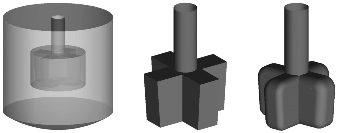
The normal model, the standard impeller, and the worn impeller, respectively.

Obtaining of simulation data

In order to obtain the data of the transient flow field, we chose several rectangular areas as inspection regions and then exported the data locating in the inspection regions at each step. Figure 2 shows the position of inspection regions; there was one inspection region in the normal and worn models, while two opposite inspection regions were set up in the eccentric model. Four inspection regions lay in the XZ plane and possessed the equivalent clearance from the sliding face.

Figure 2.

Position of inspection regions: (a) lain in the normal and worn models and (b) lain in the eccentric model.

Fixed time step-size was set to 1e−04 s when the calculation converged, and recording data began at one of the blades past the inspection plane about 43°. Ultimately, a total of 600 velocity fields were acquired for each model. The inspection regions in the normal and worn models contain 684 nodes, while the number of nodes varies slightly for the distortion on the inspection regions in the eccentric model.

Results and discussion

Macroscopic flow field

Three models have similar macroscopic flow field; thus, we only analyzed that of the normal model. Figure 3 shows the velocity vector on the axial section of the normal model, and two features can be found as follows:

Molten iron flowed in from the upper and lower regions of the impeller and came out from the cylinder surrounding the impeller, which is the main flow in the ladle.

Two pronounced vortexes appeared near the outer edge of the blades on the top and bottom of the impeller.

Figure 3.

Velocity vectors on the axial section (the normal model).

The motion of molten iron in the ladle was driven by the impeller; the first feature indicates that the rotation speed needs to increase with the growing of the wear of the impeller in order to achieve approximate hydrodynamic conditions. The vortex in the second feature is beneficial to the spread of flux, so the strength of the vortex affects the desulfurization efficiency.

To identify and characterize the flow structures in the ladle, the POD was performed on the data of the velocity field. The velocity field is 3D in the ladle; however, the analysis was limited to a 2D plane, and only both radial and axial velocity data were used. The eigenfunction corresponding to the first mode is plotted in Figure 4(a), where the horizontal and vertical axes represent the node number in the inspection region along the X- and Z-directions, respectively, and the axes in the next chart of the streamline pattern have same meanings. The instantaneous velocity field associated with the first mode is given by

V_{k} (x, z, t) = a_{k} (t) \times ϕ_{k} (x, z) (k = 1)

(4)

where $a_{k} (t)$ is the temporal coefficient and $ϕ_{k} (x, z)$ is the spatial model.

Figure 4.

First POD mode: (a) eigenfunction, (b) comparison between the first mode and mean flow, and (c) pdf of $a_{1} / sqrt (λ_{1})$ .

The vertical average profile of the horizontal component of the velocity field reconstructed with the first mode is compared to that of the mean flow in Figure 4(b). The two profiles are approximately identical. Indeed, the velocity field associated with the first mode corresponds to the mean flow, and the mean flow is formulated by

V_{mean} = \frac{1}{N} \sum_{k = 1}^{N} V_{k} (x, z, t)

(5)

where $V_{k} (x, z, t)$ is the kth instantaneous velocity field.

In POD technique, the follow formula is valid

\frac{1}{N} a_{i} a_{j} = λ_{i} δ_{ij}

(6)

where $a_{i}$ and $a_{j}$ are the temporal coefficients corresponding to the ith and jth eigenfunctions, respectively, and $λ_{i}$ is the ith eigenvalue, and N is the number of samples.

The coefficient a₁ mentioned in equation (4) is the temporal coefficient corresponding to the first eigenfunction, and Figure 4(c) shows the probability density function of the coefficient a₁ which was normalized by the square root of the first eigenvalue $λ_{1}$ . Two key points can be seen from Figure 4(c). The first is that the value of $a_{1} / sqrt (λ_{1})$ is relatively centered on 1, which reflects that the first mode is predominant in the flow field, while the second is that the distribution of the coefficient a₁ shows a dispersion trend, which reflects that there exists a relatively large fluctuation about the concentration of the first mode in the flow field.

Mode analysis

Figure 5 shows the streamline patterns of the first mode of three models, and the background presents the vorticity. In the worn model, the decreasing diameter of the impeller due to continuous wear resulted in the region shrank of the vortexes and made the inspection region away from the vortexes, which caused the vorticity to be lower than that of the other models, and it can be observed from Figure 5. The region shrank of the vortexes has a negative effect for the desulfurization; thus, the impeller needs to be replaced when the shrink reaches a certain level to keep favorable hydrodynamics. The pattern of the small spacing in the eccentric model is slightly different from that of others, compared with other models, the curvature of streamline on the middle of ladle nearly the wall is larger for the radial velocity of molten iron is greater due to the impeller being nearer to the wall.

Figure 5.

Streamline patterns of the first mode: (a) the normal model, (b) the worn model, (c) the eccentric model with large spacing, and (d) the eccentric model with small spacing.

The eigenvalues of the first 20 modes normalized by the sum of eigenvalues are plotted in Figure 6, which reflects the relative contribution of the modes to the total kinetic energy of the flow field. As seen from Figure 6, the magnitude of the eigenvalues rapidly reduces with the increase in mode number, and the first mode explains more than 90% of the energy. The third eigenvalue in the worn model decreases with a faster rate compared with the other models, which is related to the flow structure corresponding to the third mode. Examining the four curves in Figure 6, it can be inferred that the large structure in the flow field can be well reconstructed using the linear combination of the first three modes, and the later higher modes can be considered as the turbulence and chaotic.

Figure 6.

Eigenvalues of the first 20 modes.

Figure 7 displays the second and third modes of three models. The ambient fluid was entrained by the moving mean flow; thus, it can be considered that the second mode was partly induced by the first mode. Combined with the first mode in Figure 5, the first and second modes disclose the upper and lower large eddies, which are the largest structure in flow field in the ladle. Meanwhile, the strength and fluctuation of the first mode raise the distinction of the second mode between three models. The third mode intuitively reflects the structure of the vortexes on the upper and lower regions of the impeller that also is partly revealed in the second mode. The strength and size of the vortexes in the worn model are least among three models; the possible reason is that the proportion of the third eigenvalue in the sum of eigenvalues is lower compared with other models. Three models in general have two vortexes distributed in the ambient of the impeller, and we can seen that the size of the upper vortex is slightly larger than the lower vortex except in the worn model since the upper diameter of the impeller is a little larger than the lower. In the worn model, the two vortexes are not significantly different due to the nearly identical diameters caused by the abrasion on the blades.

Figure 7.

Streamline patterns of the second and third modes: (a) the normal model, (b) the worn model, (c) the eccentric model with large spacing, and (d) the eccentric model with small spacing.

Observing the third mode carefully, we can find that there are two obscure vortexes on the top and bottom of the inspection regions and their rotation direction is opposite to that of the middle vortexes as shown in Figure 7 about Mode 3. The development of these two vortexes is not quite identical in three models, which illustrates the difference of flow field among models.

As mentioned previously, the first two modes are related to the large size structure of the flow field; thus, their coefficients might have a possible relation. Figure 8 shows the correlation between the first two mode coefficients, where a₁ and a₂ are the temporal coefficients corresponding to the first and second eigenfunctions, respectively.

Figure 8.

Correlation map of the first two mode coefficients: (a) the normal model, (b) the worn model, (c) the eccentric model with large spacing, and (d) the eccentric model with small spacing.

The circle represents the first 190 data of two coefficients, and the data from 191st to 340th are identified as solid point, and the rest mark by cross in Figure 8. Recording data started at one of the blades (blade 1) past the inspection plane about 43°, and the impeller turned about 145° and another blade (blade 2) passed through the inspection plane during recording data. It can be considered that the large-scale structure reached a stable state at the beginning of data collection (the circle in Figure 8), and then the stable state of the structure transited from one to another after blade 2 turned past the inspection plane, and the solid point represented the intermediate state. The correlation between the sample number and the turned angle of the impeller is plotted in Figure 9. Compared with Figure 8, a definite relative relation between the coefficients a₁ and a₂ can be clearly seen. Blade 1 was about 89° from the inspection plane and blade 2 nearly located on the inspection plane at the sample number 191; therefore, the a₁–a₂ relation began to change at the moment. At sample number 341, blade 2 left the inspection plane and then the a₁–a₂ relation entered another stable state.

Figure 9.

Correlation between the sample number and the turned angle of blade 1 relative to inspection plane.

The correlation map of the coefficients a₁–a₂ in the worn model is different from the others in Figure 8; the possible reason is that the effect of the mean flow weakens on the entire flow field due to the wear on the blades.

Liné et al.¹⁷ showed that the phase portrait about a₂–a₃ is an ellipse, where a₃ is the temporal coefficient corresponding to the third eigenfunction, and they can thus be related by the expression

\frac{a_{k}^{2}}{2 λ_{k}} + \frac{a_{k + 1}^{2}}{2 λ_{k + 1}} = 1 (k = 2)

(7)

Figure 10 shows the correlation map of the coefficients a₂–a₃, and it can be seen that only the shape in the worn model is close to ellipse. In the study by Liné et al., the D/T is equal to 0.33 and the Reynolds number is equal to 530 in their experiment, but these values are 0.42 and 1.13e05, respectively, in the simulation. It can be concluded by a comparative analysis that the development of the vortexes is restricted in space and dynamic (the decreased viscosity) by a high D/T and Reynolds number, which results in that the shape of the coefficients a₂–a₃ deviates from an ellipse. In the worn model, however, the vortexes have relatively larger space to develop for the smaller diameter of the impeller, which partly manifest the shape as an ellipse. Actually, Oudheusden et al.²² pointed out that the POD modes are coupled when their POD eigenvalues are close to each other, whereas the POD eigenvalues in the article did not suffice the request.

Figure 10.

Correlation map of the coefficients a₂–a₃: (a) the normal model, (b) the worn model, (c) the eccentric model with large spacing, and (d) the eccentric model with small spacing.

The temporal variation in the second mode coefficient a₂ of three models is plotted in Figure 11(a). They show a trend of periodic variation which is the change rule of the mean flow. In the worn model, the variation strength is smaller than that of other models. Figure 11(b) shows the spectra of the coefficient a₂ for all cases. The number of samples is less which leads to low-frequency resolution; therefore, the spectra can only be used as a qualitative analysis. The main peak frequency in the worn model is 33.3 Hz, while that in other models is 50 Hz, which indicates that the fluctuation frequency of the mean flow in the worn model is less than that in other models. However, note that the rotating speed of the impeller in the worn model is the largest, which can be attributed to the fact that the diameter of the impeller has a great impact on flow field. The main peak frequency is equal in the normal and eccentric models, which indicates that the fluctuation of the mean flow has same frequency on eccentric or central stirring. Observing the magnitudes corresponding to the main peak in Figure 11(b), we can see that the magnitude in the eccentric model with small spacing is significantly greater than others, which implies that the strength of the mean flow in that inspection region is stronger than others. In contrast, the magnitude in the eccentric model with large spacing is the smallest, which implies that its mean flow is the weakest. The coefficient time series of the worn model fluctuates smoothly, so an evident second peak does not appear yet that appears in other spectra, which means that the variation in flow field in the worn model is smoother than that in other models. That can be partly reflected from Figure 6, since the eigenvalues from the third mode in the worn model fall faster than that in other models.

Figure 11.

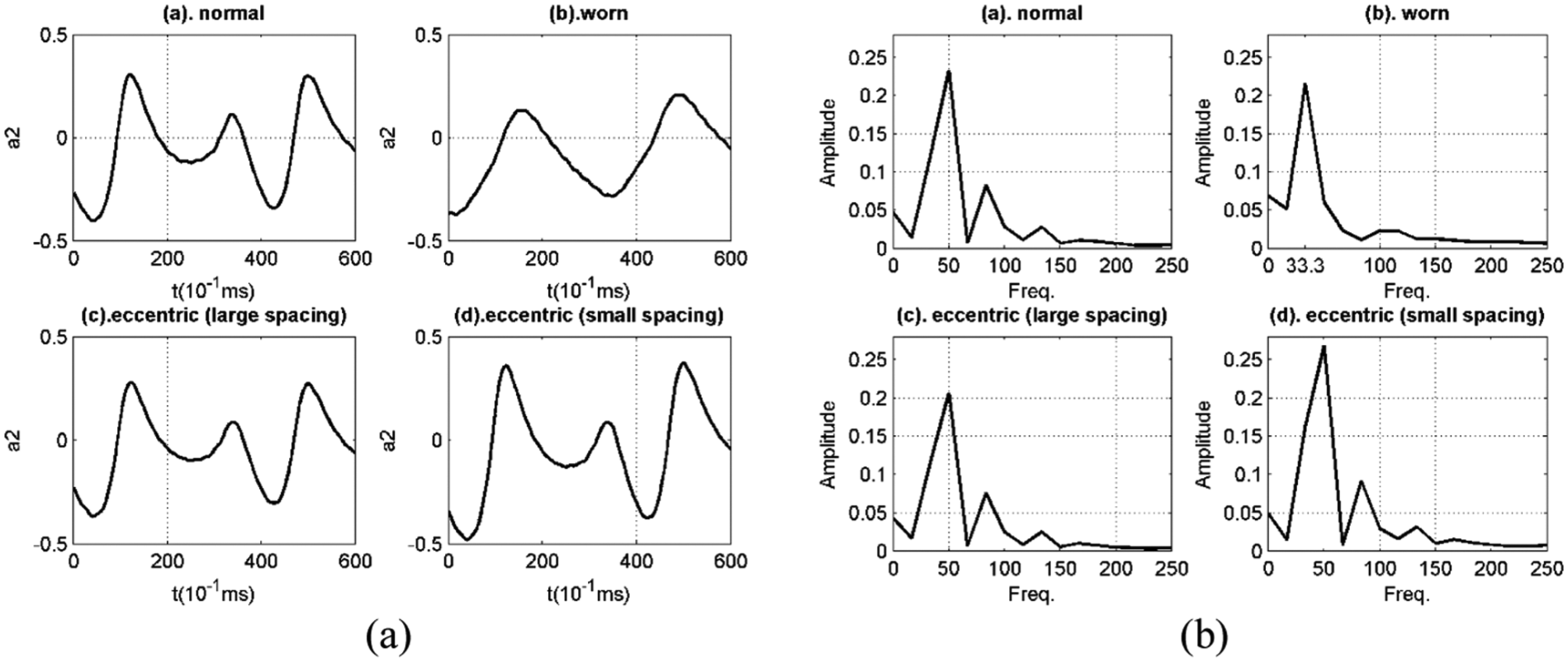
Second POD mode coefficients: (a) time series and (b) the spectra.

Figure 12 shows the fourth mode of three models. The streamline patterns are similar except that in the eccentric model with large spacing. There are two obvious vortexes in Figure 12(c) and that are advantageous to mixing, which also explains that eccentric stirring profits the desulfurization to some extent.

Figure 12.

Streamline patterns of the fourth mode: (a) the normal model, (b) the worn model, (c) the eccentric model with large spacing, and (d) the eccentric model with small spacing.

Conclusion

The numerical simulation was carried out on three scaled-down models of the desulfurization. A total of four inspection regions were set up to collect the data of flow field, and the data were processed by POD technique and then the characteristics of the stirring flow field were analyzed based on the result of the POD treatment. The main conclusions are as follows:

The first mode represents the mean flow that has a relatively large fluctuation in flow field despite having a high proportion in total kinetic energy.

The second mode is partly induced by the first mode, a nearly approximate linear relation obviously exists between them, and the state of the stable relation changes during the stirring process.

The change in the mean flow in the worn model is slow compared with other models in spite of having a larger rotation speed according to the spectrum of the second mode coefficients.

The patterns of the flow field on two sides in the eccentric model are greatly different, and the asymmetry caused by eccentricity brings more different POD modes for the flow field, which is benefit to the effect of desulfurization.

Footnotes

Academic Editor: Chin-Lung Chen

Declaration of conflicting interests

The author(s) declared no potential conflicts of interest with respect to the research, authorship, and/or publication of this article.

Funding

The author(s) disclosed receipt of the following financial support for the research, authorship, and/or publication of this article: This work was supported by National Natural Science Foundation of China (No. 51475340) and the Science and Technology Support Program of Hubei Province (No. 2014BAA097).

References

Kurokawa

Matsuo

Jouguchi

. The development in hot metal desulphurization process. Sumitomo Met 1993; 45: 52–58.

Yugov

Romberg

AL.

Improving the quality of pig iron and steel. Metallurgist+ 2003; 47: 62–65.

Scargiali

Busciglio

Grisafi

. Oxygen transfer performance of unbaffled stirred vessels in view of their use as biochemical reactors for animal cell growth. Chem Eng Trans 2012; 27: 205–210.

Scargiali

Busciglio

Grisafi

. Influence of viscosity on mass transfer performance of unbaffled stirred vessels. Chem Eng Trans 2013; 32: 1483–1488.

Yang

Zhou

SJ.

Effect of gravity on the hydrodynamics in an unbaffled stirred vessel. Chem Eng Technol 2015; 38: 819–826.

Montante

Bakker

Paglianti

. Effect of the shaft eccentricity on the hydrodynamics of unbaffled stirred tanks. Chem Eng Sci 2006; 61: 2807–2814.

Galletti

Pintus

Brunazzi

Effect of shaft eccentricity and impeller blade thickness on the vortices features in an unbaffled vessel. Chem Eng Res Des 2009; 87: 391–400.

Hidalgo-Millan

Soto

Zenit

. Effect of eccentricity on the pumping capacity in an unbaffled vessel. Can J Chem Eng 2011; 89: 1051–1058.

Smit

Düring

Vortex geometry in stirred vessels. In: Proceedings of the Seventh European congress on mixing, Brugge, 18–20 September 1991, pp.633–639.

10.

Lamarque

Zoppé

Lebaigue

. Large-eddy simulation of the turbulent free-surface flow in an unbaffled stirred tank reactor. Chem Eng Sci 2010; 65: 4307–4322.

11.

Busciglio

Caputo

Scargiali

Free-surface shape in unbaffled stirred vessels: experimental study via digital image analysis. Chem Eng Sci 2013; 104: 868–880.

12.

Lumley

JL.

The structure of inhomogeneous turbulent flows. In: Yaglom

Tatarski

(eds) Atmospheric turbulence and radio wave propagation, vol. 13. Moscow, Russia: Nauka, 1967, pp.166–178.

13.

Sirovich

Turbulence and the dynamics of coherent structures. Q Appl Math 1987; 45: 561–571.

14.

Tabib

Joshi

JB.

Analysis of dominant flow structures and their flow dynamics in chemical process equipment using snapshot proper orthogonal decomposition technique. Chem Eng Sci 2008; 63: 3695–3715.

15.

Moreau

Liné

Proper orthogonal decomposition for the study of hydrodynamics in a mixing tank. AIChE J 2006; 52: 2651–2655.

16.

Gabelle

Morchain

Anne-Archard

. Experimental determination of the shear rate in a stirred tank with a non-newtonian fluid: carbopol. AIChE J 2013; 59: 2251–2266.

17.

Liné

Gabelle

J-C

Morchain

. On POD analysis of PIV measurements applied to mixing in a stirred vessel with a shear thinning fluid. Chem Eng Res Des 2013; 91: 2073–2083.

18.

Wang

. POD study on large-scale structures of viscoelastic turbulent drag-reducing flow. Adv Mech Eng 2014; 6: 574381.

19.

Shi

Liu

Wan

JJ.

Influence of wall proximity on characteristics of wake behind a square cylinder: PIV measurements and POD analysis. Exp Therm Fluid Sci 2010; 34: 28–36.

20.

Rodolphe

Marianna

Emmanuel

. Phase averaged turbulence properties in the near wake of a circular cylinder at high Reynolds number using POD. Exp Fluids 2007; 43: 341–355.

21.

Greig

Siddiqui

Karava

. Investigation of fundamental flow mechanisms over a corrugated waveform using proper orthogonal decomposition and spectral analyses. Int J Therm Sci 2015; 96: 160–172.

22.

Oudheusden

BWV

Scarano

Hinsberg

NPV

. Phase-resolved characterization of vortex shedding in the near wake of a square-section cylinder at incidence. Exp Fluids 2005; 39: 86–98.

Numerical study of flow field on molten iron desulfurization with mechanical stirring

Abstract

Keywords

Introduction

Numerical simulation arrangement

Simulation model

Obtaining of simulation data

Results and discussion

Macroscopic flow field

Mode analysis

Conclusion

Footnotes

Declaration of conflicting interests

Funding

References