
Abstract
The Monte Carlo simulation method for turbomachinery uncertainty analysis often requires performing a huge number of simulations, the computational cost of which can be greatly alleviated with the help of metamodeling techniques. An intensive comparative study was performed on the approximation performance of three prospective artificial intelligence metamodels, that is, artificial neural network, radial basis function, and support vector regression. The genetic algorithm was used to optimize the predetermined parameters of each metamodel for the sake of a fair comparison. Through testing on 10 nonlinear functions with different problem scales and sample sizes, the genetic algorithm–support vector regression metamodel was found more accurate and robust than the other two counterparts. Accordingly, the genetic algorithm–support vector regression metamodel was selected and combined with the Monte Carlo simulation method for the uncertainty analysis of a wind turbine airfoil under two types of surface roughness uncertainties. The results show that the genetic algorithm–support vector regression metamodel can capture well the uncertainty propagation from the surface roughness to the airfoil aerodynamic performance. This work is useful to the application of metamodeling techniques in the robust design optimization of turbomachinery.
Keywords
Introduction
Almost all of the real-world engineering systems suffer from a wide variety of uncertainties, such as manufacturing tolerance, material nonuniformity, mathematical and/or numerical approximation, environment variation, and in-service degradation. Due to the lack of proper treatment of these uncertainties, design engineers have seen too many unpleasant cases of performance deficiencies in their own products. It does pose a significant challenge for engineers to include rigorous uncertainty analysis as much as possible within the cycle of design to make cost-effective products. 1
The primary task of the uncertainty analysis is to evaluate the impact of various uncertainties on the performance of the product, in which both deterministic simulations and statistical analysis are required. According to the manners by which the deterministic solvers are implemented with the statistical methods, the approaches of uncertainty analysis are classified into two groups: the intrusive methods and the nonintrusive methods. 2 The former, such as the polynomial chaos (PC) techniques, can directly yield the uncertain outputs through a one-time solution of certain reformulated equations; however, they are severely limited to low-dimensional, low-order, and short-time systems due to the mathematical and/or numerical difficulties arising from the reformulated equations. The latter, such as Monte Carlo simulation (MCS) method or its variants, are often easy to implement in combination with the available deterministic solvers, yet requiring a huge number of simulations for a statistical convergence.
Modern engineering analysis and design are frequently based on high-fidelity simulation tools such as the computational fluid dynamics (CFD) for fluid flow and the finite element analysis (FEA) for structural strength and vibration. These high-fidelity simulation tools are often difficult, if not impossible, to be directly used for the uncertainty analysis and design due to the heavy computational load in spite of the continuing advances of computing power. The MCS-based uncertainty analysis would be prohibitively expensive because of the requirements of even more CFD and/or FEA simulations of sampling points. An efficient measure to tackle this issue is to build variable-fidelity metamodels, which are regarded as a “model of the model,” 3 that is, a fast, inexpensive, effective but approximate model of the high-fidelity model. So far, various metamodels have been developed, such as polynomial regression (PR), 4 Kriging (KG), 5 multivariate adaptive regression splines (MARS), 6 artificial neural network (ANN),7,8 radial basis function (RBF),9,10 and support vector regression (SVR).11,12 Due to the greatly reduced computational cost, the metamodeling techniques have been widely used for the analysis and design of engineering devices.13,14 Typically, the applications of metamodeling techniques in turbomachinery design and analysis can be found in Chahine et al., 15 Mackman et al., 16 Sugimura et al., 17 Ma et al., 18 and Ju and Zhang. 19
One of the most important issues in metamodeling engineering problems is to evaluate the performances of metamodels and then select the most appropriate one for their design and analysis. Jin et al. 20 performed a systematic comparison among PR, KG, MARS, and RBF. They aimed at developing standard procedures and multiple criteria for metamodel evaluation. In the following studies, some other metamodels were also compared in some particular applications.16,21–25 All these comparative studies, to some extent, revealed the great potential and promise of ANN, RBF, and SVR for approximation. These three models are acknowledged as the artificial intelligence (AI) metamodels, which allow the behavior of self-learning and can smartly extract the mechanisms that underlie the complex systems. However, it remains unknown yet which of them has the best approximation capability in general cases and whether they could be used for turbomachinery uncertainty analysis. Therefore, in this study, an intensive comparison among these three AI metamodels was particularly conducted, where the performance evaluation strategies were carefully designed and tested through a total of 10 nonlinear functions with different problem scales and sample sizes.
Additional efforts were then devoted to applying the AI metamodeling technique to the uncertainty analysis of a wind turbine airfoil. As exposed to harsh environmental conditions, the in-service wind turbine blades unavoidably suffer from insect and/or dust contaminations, blade erosion and/or corrosion, and massive sand build-up, which cause increased blade surface roughness to varying degrees. So far, extensive numerical and experimental studies have concluded that the increased surface roughness, in particular around the blade leading edge (LE), can induce boundary layer disturbances, earlier turbulence transition and eventually wind turbine performance degradation.26–31 However, most of these studies only obtained deterministic results and ignored the wind turbine performance variations due to the stochastic nature of the surface roughness in real conditions. In view of this, the motivation of the present uncertainty analysis was to investigate the impact of surface roughness uncertainties on the aerodynamic performance of a wind turbine airfoil, although the used methodology can be extended without modifications to other types of uncertainties.
This article is organized as follows. Section “AI metamodels” mainly presents the basic formulations of the three AI metamodels: ANN, RBF, and SVR. In section “Numerical assessment of metamodeling performance,” a total of 10 analytical functions are tested to compare these three AI models in terms of accuracy and robustness, where the impacts of problem scale and sample size are carefully examined. The focus of section “Uncertainty analysis of wind turbine airfoil” is on the application of the metamodeling techniques to the uncertainty analysis of a wind turbine airfoil under surface roughness uncertainties. Some conclusions are drawn in section “Conclusion.”
AI metamodels
ANN
The mathematical form of an ANN model with one hidden layer and one output neuron can be written as 7

where
As demonstrated in our previous work, 19 the initial weights used in the BP algorithm are often difficult to determine but significantly affect the ANN performance. These parameters are thus taken as the predetermined ones and optimized by the genetic algorithm (GA), as will be discussed in section “Use of GA.”
RBF
The mathematical form of a RBF can be written as9,10

where
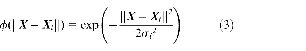
where
During the learning procedure of a RBF model, the predetermined parameters are the spread factors in equation (3) and the initial weights in equation (2).
SVR
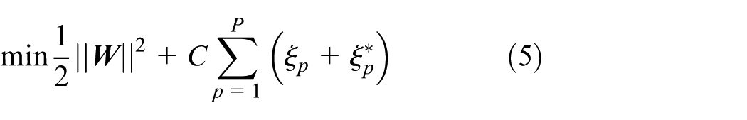
With the concept of

where

where
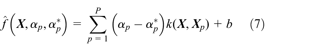
where
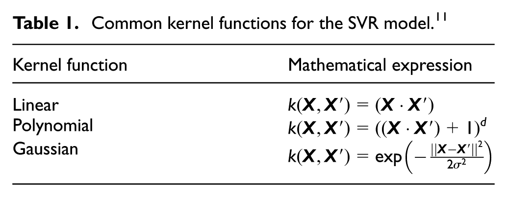
Common kernel functions for the SVR model. 11
Use of GA
The approximation performances of AI metamodels are closely associated with the predetermined parameters, which in most studies were specified or adjusted randomly. This may be less convincing or even misleading in that method A with a good set of parameters is likely to achieve better approximations than method B with a poor set of parameters even if method B is generally more accurate than method A. With this in mind, Li et al. 24 employed the hold-out validation plus grid search scheme to optimize the predetermined parameters of metamodels. However, this scheme is time-consuming and only limited to discrete parameter values. By contrast, modern evolutionary algorithms, for example, GA, can be more efficient and versatile for finding out the global optimums.
In this work, GA was adopted to optimize the predetermined model parameters through minimizing errors between the metamodel outputs and the actual outputs, the motivations behind which are twofold: first, it eliminates the uncontrollable randomness in the modeling process and thus enhances the metamodel training efficiency and robustness; second, GA helps to maximize the approximation accuracy of each metamodel, which thus strengthens the fairness of comparison in the following section.
Here, it has to be remarked that the GA parameters were tuned for different metamodels and different test cases. Detailed implementations of GA in metamodel optimization can be found in Ju and Zhang. 19
Numerical assessment of metamodeling performance
Descriptions of test problems
So far, the number of independent design variables is generally limited below 10 in the simulation-based and metamodel-assisted design optimization of turbomachinery.13,16–18 A total of 10 analytic functions with different degrees of nonlinearity and problem scales22,32,33 were first chosen in this section for a comprehensive evaluation of the three AI metamodeling techniques. Among them, the first six functions have not more than three independent variables and were classified as small-scale problems, while the other functions with 5, 8 or 10 variables were large-scale problems in this study. The mathematical expressions of these functions are listed in Appendix 1.
The training sample sets were generated by means of the uniform design of experiment (DOE), which is capable of providing fewer training samples with better uniformity and representativeness. 34 In a uniform DOE table Un(tq), n denotes the number of experiments or the sample size while q and t represent the number of factors (i.e. variables) and their levels, respectively. Accordingly, different training sampling sets were generated for different functions, that is, small and large sample sets for small-scale problems, while scarce, small, and large sample sets for large-scale problems (see Table 2). In summary, totally 6 × 2 + 4 × 3 = 24 training sample sets were generated for approximation. Here, the terms “scarce,”“small,” and “large” did not denote fixed values but were defined with respect to the problem scale, that is, the factor q in the uniform DOE table. Besides the training sampling sets, additional 10 testing sample sets were randomly generated within the variation ranges to verify the approximation performance.
Training and testing sample sizes for different problems.

Performance measures
To evaluate the approximation performance of the metamodels, a group of measures have been developed, such as accuracy, robustness, efficiency, transparency, and simplicity. 21 Among them, accuracy and robustness were the primary focus of this study because they play essential roles in determining whether a metamodel is acceptable or not for approximation.
Accuracy
Accuracy is defined as a metamodel’s capacity of predicting the system response over the pre-specified design space. To take a comprehensive measure of a metamodel’s accuracy performance, three error metrics described in equations (8)–(10) were investigated, that is, root mean square error (RMSE), averaged absolute error (AAE), and maximum absolute error (MAE) 21


The above errors should be calculated from testing samples rather than training samples. Among them, N denotes the number of testing samples,
Considering the different output ranges for the 10 test functions (see Appendix 1), it is necessary to normalize the obtained error metrics to facilitate the comparison among the three metamodels across various approximation problems. For each metamodel’s error metrics for a test function, two types of normalizations were defined in this study:
Normalization 1

Normalization 2

where

Two other mean values,
Robustness
Robustness measures a metamodel’s capacity of achieving similar accuracies for different approximation problems. Mathematically, here it was defined as the standard deviation of error metrics across all the problems of interest

Two other standard deviations,
Comparison results
Overall performance
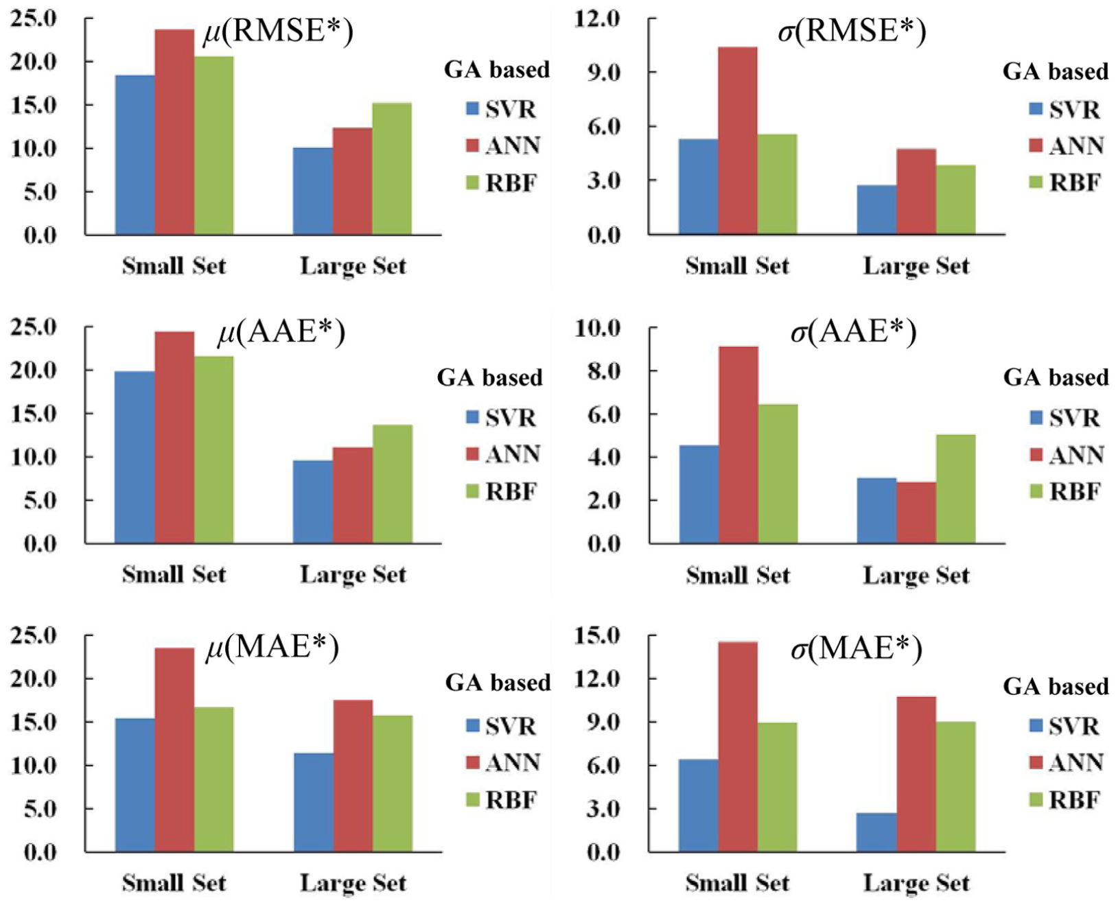
The overall performances of the GA-based AI (GA-AI) metamodeling techniques were calculated as follows: for each metamodel, Normalization 1 (equation (11)) was first implemented to calculate its
The corresponding results are illustrated in Figure 1. Compared with the other two metamodels, the GA-based SVR (GA-SVR) achieved both lower mean values and lower standard deviations of the

Overall performance comparison among the three metamodels: (a) mean values and (b) standard deviations.
Impact of problem scale
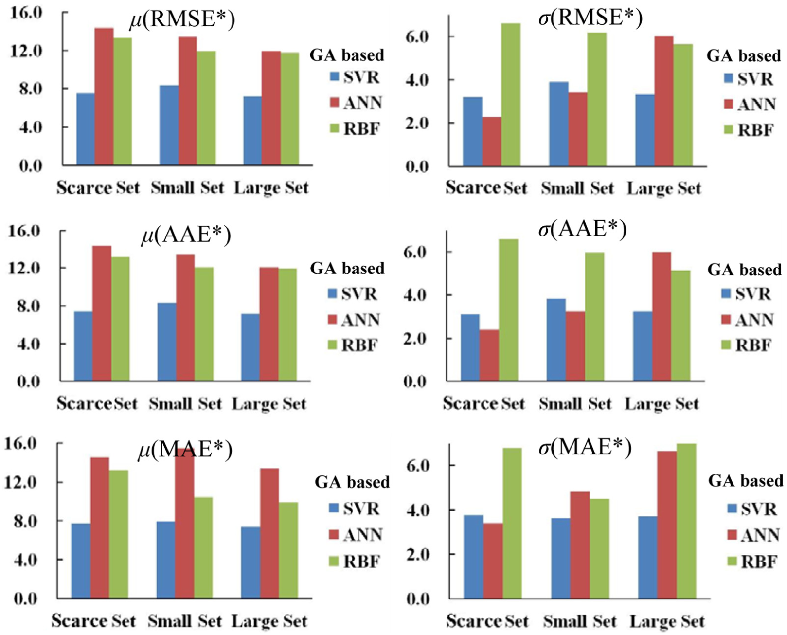
To examine each GA-AI metamodel’s performances in approximating problems with different scales, Normalization 1 (equation (11)) was adopted, while a different averaging strategy from the above was used: for each metamodel, the mean values and standard deviations of errors were calculated first for small-scale functions through averaging across a total of 6 × 2 = 12 approximation problems (i.e. the small and large sample sets for each of the first six functions); and then, the average was performed for large-scale functions across the 4 × 3 = 12 approximation problems (i.e. the scarce, small and large sample sets for each of the last four functions). The comparison results are given in Figure 2.

Performance comparison among the three metamodels for problems with different scales.
Except for the
Impact of training sample size
To further investigate the impact of training sample size on the performance of metamodels, particular attention was paid to the approximation results under different training sample sets. First, the values of RMSE*, AAE*, and MAE* were obtained using Normalization 2 (equation (12)), by which the best combination of the metamodel and sample size could be obtained for each test function. Second, for each group of the small- and large-scale test functions, more detailed average was performed across approximation problems with the same type of sample set.
Figure 3 summarizes the performances of the three GA-AI metamodeling techniques with different sample sets for small-scale problems. GA-SVR generally performed the best in spite of a slight inferiority in
Performance comparison among the three metamodels for small-scale problems under different sample sizes.
Compared with the small-scale problems, the large-scale problems were less influenced by sample sizes (see Figure 4). This is interesting and encouraging due to the absence of the great expense for getting the large sample information. The averaged accuracies of GA-SVR were almost equivalent for the three kinds of sample sets, while significantly better than those of the other two metamodels. GA-RBF achieved the second best accuracy performance, followed by GA-ANN. In terms of the robustness performance, GA-SVR still performed excellently for all the sample sets. GA-ANN was the most robust metamodel for the scarce and small sample sets but its performance deteriorated significantly when the sample size became large. GA-RBF achieved the worst robustness performance in the group. Therefore, the combination of the GA-SVR metamodel and a scarce sample set could be acceptable for approximating large-scale problems. For most practical problems, the most time-consuming part during the metamodeling process is spent on the evaluation of training samples rather than the model construction itself. From this point of view, GA-SVR metamodel could be the most efficient selection for an accurate approximation of the large-scale problem.
Performance comparison among the three metamodels for large-scale problems under different sample sizes.
In summary, SVR showed generally the best approximation performance in terms of accuracy and robustness among the three AI metamodels for the tested mathematical cases. The strong generalizability of SVR can be attributed to the structural risk minimization (SRM) inductive principle which strikes a good balance between the empirical risk and problem complexities. 12
Uncertainty analysis of wind turbine airfoil
In this section, the above-mentioned GA-SVR metamodeling technique has been applied to the uncertainty analysis of a wind turbine airfoil under surface roughness uncertainties. The airfoil to be investigated was FX 63-137. 35 Prior to the uncertainty analysis, the deterministic CFD solver was outlined in the next subsection.
Deterministic CFD simulation
CFD model
The deterministic aerodynamic performances of both smooth and rough airfoils were obtained by numerical solution of two-dimensional steady incompressible Reynolds-averaged Navier–Stokes equations using a finite-volume method solver, Fluent 6.3. The pressure-based SIMPLEC algorithm was employed to treat the flow velocity–pressure coupling. The convection terms of the governing equations were discretized by the second-order upwind scheme and the diffusion term by the second-order central difference scheme. The shear-stress transport (SST) k-ω model was used to close the turbulence terms, in which the calculation of turbulence vorticity ω near solid wall carefully considers the surface roughness height ks. To consider the effect of surface roughness, this turbulence model requires that the computational grid near the rough surface should be fine enough to include the roughness height ks, and the y+ of the first nodes near the rough surface should be kept below unit.
The inlet boundary of the computational domain was placed at the location about 12.5 chord-length upstream of the airfoil and the outlet was at about 20 chord-length downstream of the airfoil. The boundary condition at the inlet was the free stream flow velocity, while a static pressure was specified at the outlet. The nonslip wall boundary condition was applied on the airfoil surface. As shown in Figure 5, the generated computational grids comprised the C-type grids around the airfoil and the H-type grid in the far field region. The area-averaged y+ of the first nodes close to the airfoil surface was about 0.89. The number of nodes assigned inside the boundary layer was 15. Besides, the grid independency was examined via successively increasing the grid number along the airfoil surface until the evaluated aerodynamic quantity was essentially no longer changed. Finally, the total number of grid nodes was 153 on the airfoil surface and 42571 all over the computational region.

Local grids around the wind turbine airfoil.
Note that the capacity of the above CFD model in predicting the airfoil performance in both clean and rough conditions has been validated by Ferrer and Munduate 28 in their work. In this study, the CFD model was directly employed to evaluate the effect of surface roughness on the aerodynamic performance of the FX 63-137 airfoil.
Performance comparison
As shown in Figure 6 (top), the rough airfoil to be investigated was assumed to have deterministic roughness zones uniformly distributed around LE, and the roughness height (ks) was fixed to be 0.3 mm, covering 20% (x/c) of the chord from the LE. The airfoil chord was 305 mm in this study. In Figure 6 (down), the calculated aerodynamic performances of the rough airfoil were characterized by a reduced lift and an increased drag relative to the smooth one. The performance deteriorations became more apparent as the incidence angle increased. The maximum lift coefficient was reduced by 4.8%, while the related drag coefficient had a relatively small increase of about 1.9%, in comparison with the clean airfoil. In addition, the stall incidence angle of the rough airfoil shifted from 12° to 11°, indicating the occurrence of an earlier stall.

Comparison of the lift-drag performance between the smooth and rough airfoils.
Figure 7 shows the calculated pressure distributions of the smooth and rough airfoils at near-stall points. As can be seen, the most remarkable difference between smooth and rough airfoils was the flow behavior near the LE on the suction surface (SS): the rough airfoil showed a much weaker velocity acceleration from the LE, corresponding to a thicker boundary layer on the airfoil surface. This gives rise to the deteriorated airfoil performance with reduced lift, increased drag, as well as earlier stall.

Comparison of the pressure coefficients Cp between the smooth and rough airfoils.
Stochastic roughness model
To quantify the stochastic nature of the surface roughness distributed on the airfoil surface, two stochastic models were built based on the Gaussian probability distributions and the B-spline function, respectively. In the first model, the surface roughness distributions on the airfoil were assumed to be spatially uniform, while the uniformly distributed roughness height ks and the dimensionless covering length x/c were considered to be randomly varied, both following the Gaussian probability distributions, as shown in Figure 8. Compared with the first model, the second one is more irregular and thus closer to the real conditions. As shown in Figure 9, this model used the random-shaped B-spline curve to characterize the nonuniformity of the surface roughness distribution around the airfoil LE. The interpolating points of the B-spline curve were supposed to be randomly varied around the mean value, and any negative values on the curve were reassigned to be zero to simulate the abrupt transitions between the rough and smooth regions in real conditions. The roughness parameters of both models had the same variation ranges: the roughness height ks was from 0 to 0.42 mm and the dimensionless covering length x/c varied from 0 to 0.3.

Gaussian probability distributions of the surface roughness parameters: (a) roughness height and (b) dimensionless covering length.

Roughness distribution by B-spline curve.
Uncertainty analysis and results
In order to alleviate the huge computational cost in the uncertainty analysis by MCS, the GA-SVR metamodels presented in the previous sections were constructed to fast predict the
Case 1: Gaussian probability distribution
The first uncertainty analysis concerned the roughness uncertainties shown in Figure 8. A total of four uncertain inputs were considered, that is, ks and x/c for each of the SS and pressure surface (PS) of the wind turbine airfoil. Therefore, this case was classified as a small-scale case.
A GA-SVR model was constructed to link the four roughness uncertain parameters and the
Once the GA-SVR model was built, it was integrated with the MCS method to conduct the uncertainty analysis. To further investigate how roughness uncertainties affect the
Different parameter combinations and numerical results of the uncertainty analysis in Case 1.

MCS: Monte Carlo simulation; CFD: computational fluid dynamics; SS: suction surface; PS: pressure surface.
The calculated probability distributions of
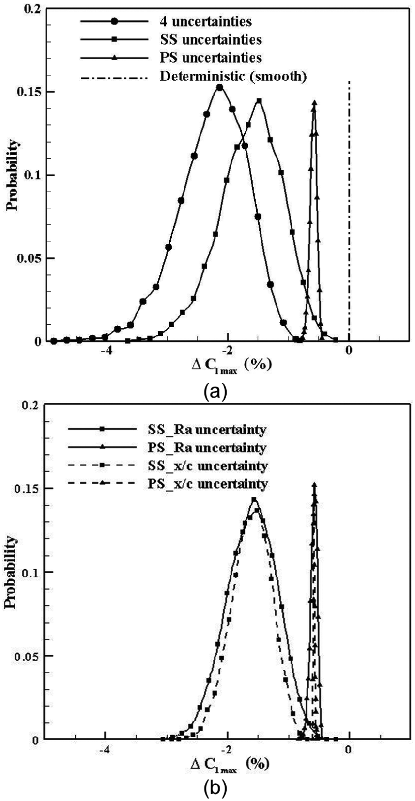
Probability distributions of the
According to the above results, the SS roughness distributions are the primary uncertainties that affect the aerodynamic performance and should be focused on in the future design and analysis of the wind turbine airfoil.
Case 2: B-spline distribution
In this case, the uncertainty analysis was based on the second model shown in Figure 9, which highlights the nonuniformity and randomness of the surface roughness distributed around the wind turbine airfoil LE. Given the results obtained in Case 1, here primary attention was focused on the SS roughness uncertainties. The eight interpolating points of the B-spline curve were taken as uncertain inputs in this analysis.
A second GA-SVR model was required to build up the relationship between the eight roughness uncertain parameters and
Table 4 shows the numerical results of this uncertainty analysis, and the resulting probabilistic distribution of
Numerical results of the uncertainty analysis in Case 2.

MCS: Monte Carlo simulation; CFD: computational fluid dynamics.

Probability distribution of
Above all, the GA-SVR metamodel can capture well airfoil performance variations due to different surface roughness uncertainties, which demonstrates the potential applicability of the GA-SVR metamodel in turbomachinery uncertainty analysis and provides reference for the future robust design optimization.
Conclusion
An intensive comparison has been conducted among three AI metamodeling techniques, that is, SVR, ANN, and RBF, of which the predetermined parameters were optimized using the GA method for the sake of a fair comparison. The metamodel performance evaluation strategies were carefully designed with the consideration of problem scales and sample sizes and tested by a total of 10 analytic functions. The GA-SVR metamodel was found to have the most accurate and robust performances for almost all the cases examined. It has to be remarked that the effect of noise on algorithm performance was not considered in this study, which, however, is worth studying in the future work.
The GA-SVR metamodel has been combined with the MCS method to conduct the uncertainty analysis of the wind turbine airfoil. For the investigated roughness uncertainty quantifications, the GA-SVR was capable of capturing the effect of surface roughness uncertainties on the aerodynamic performance of the wind turbine airfoil. This uncertainty analysis method based on GA-SVR and MCS is fairly generic. Work concerning the application of GA-SVR metamodel combined with MCS method for multi-objective robust design optimization of turbomachinery is currently ongoing.
Footnotes
Appendix 1
Academic Editor: Amir Alavi
Declaration of conflicting interests
The author(s) declared no potential conflicts of interest with respect to the research, authorship, and/or publication of this article.
Funding
The author(s) disclosed receipt of the following financial support for the research, authorship, and/or publication of this article: the work was supported by the National Natural Science Foundation of China (Grant No. 51406148) and the Postdoctoral Scientific foundation of China (Grant No. 2014M552444).