
Abstract
The primary objective of this study is to identify the characteristics of vehicle headway on multi-lane freeway under lane management in China considering car–truck interaction. More specifically, the study focused on answering the following two questions: (1) whether the car–truck interaction has impact on headway, that is, headway varies by different leading and following vehicle types and (2) what is the best-fitted distribution model for particular headway type under lane management. The team collected traffic data, including traffic flow rates, percentage of trucks, speeds, headways, and so on from four segments of Shanghai-Nanjing freeway, Jiangsu Province in China. Then, some statistical methods were used to analyze the vehicle headway. It was found that car–car, car/truck, and truck–truck headways are significantly different from each other. Also, the traffic flow rate, percentage of trucks, and lane position were found to have an influence on the vehicle headway through the tests. Using the maximum-likelihood estimation, Kolmogorov–Smirnov test, and chi-square test techniques, the distribution models and parameter functions for each headway type were built and validated. The results showed that lognormal model is suitable for car–car and truck–truck headway types, and inverse Gaussian model fits the car/truck headway type well.
Keywords
Introduction
The vehicle headway is defined as “the time, in seconds, between two successive vehicles as they pass a point on the roadway, measured from the same common feature of both vehicles.” 1 This parameter has been studied for several years because it is one of the most important and fundamental characteristics in traffic flow. Since the value of headway is closely related to the traffic operation performance, such as road capacity, level of service, and vehicle behavior, and also has some implications in terms of the safety simulation (surrogate safety measures, traffic conflict analysis, etc.), 2 many researchers still keep studying it. Now, the headway can be analyzed in detail and accurately as much as possible due to the development of the technology. Therefore, more useful and meaningful characteristics of the traffic flow can be obtained by studying the headway specifically.
The freeway construction has greatly promoted regional, social, and economic development in China, which brings about a great traffic demand for freeway and imposes huge pressure on freeway operation. Therefore, more and more multi-lane freeways appeared instead of the two-way four-lane freeways before. Also, the lane management was implemented at the same time to improve the safety and efficiency of traffic operation. Because of the increased number of lanes and the existence of lane management, the traffic characteristics get changed significantly, especially the vehicle headway. If we would like to know the new characteristics of multi-lane freeway or calculate the capacity of multi-lane freeway much more accurately or even more, it is important to analyze the proper vehicle headway distributions.
With the economic development, the number of trucks keeps increasing and becomes an important part of freeway traffic. In China, the average truck percent is >25% in most freeway, and some even up to 60%. Because of the particularity of trucks in physical and operation characteristics (e.g. larger length and low acceleration or deceleration), trucks have a significant impact on cars. For instance, car–truck interaction will cause different reactions, gap acceptance, headway distributions, and so on. So, it is necessary to analyze the headway characteristics considering car-truck interaction.
Combining the situation of lane management and car-truck interaction, the headway characteristics are related to the vehicle type in different lanes; hence, this study mainly analyzes the vehicle type–specific headway distribution on multi-lane freeway under lane management. More specifically, the study focused on answering the following two questions: (1) whether the car-truck interaction has impact on headway, that is, headway varies by different leading and following vehicle types; and (2) what is the best-fitted distribution model for particular headway type under lane management.
After this introduction, the next section of this article reviews the vehicle headway and car-truck interaction. This is followed by the data used in this research. After that is the analysis of the vehicle headway. In the following part, the distribution model will be built and then validated. The findings are summarized toward the end of this article.
Literature review
The headway between two successive vehicles is a random variable. Having a statistics about the traffic following behavior on road, the headway distribution model can be acquired. Headway distribution model is the basis of the traffic flow modeling and microscopic simulation so that it is usually used in road capacity, lane changing, vehicle conversion factor, traffic control strategies in intersection, and so on.3–6 Today, many headway distribution models have been proposed. Representatives of the vehicle headway distribution models include the exponential distribution, 7 the Erlang distribution, 8 the lognormal distribution, 9 the inverse Gaussian distribution, 10 gamma distribution, 11 the M3 distribution, 7 and so on. There are some restrictions in the use of these distribution models because they are affected by many factors such as traffic volume, percentage of trucks, road infrastructure, weather, time, and so on. 12 Mei and Bullen 13 measured the headway in a four-lane highway and found the lognormal distribution is suitable. Luttinen 14 has found that M3 model was effective for larger vehicle headways. In practical application, many researchers thought that lognormal model should be used in analyzing the traffic flow in freeway, while M3 distribution model is better for analyzing the lane changing of vehicles. 14 Al-Ghamdi 15 performed a research on vehicle headway on the urban road in Riyadh, Saudi Arabia. From the results, he found that negative-exponential, shift-exponential, and Erlang distributions are the optimal models for low, medium, and high levels of flow, respectively.
Recently, quantifiable measures have been used to infer the influence of car-truck interaction on traffic operation. Peeta et al. proposed a concept of discomfort level for the result of car-truck interaction based on behavior analysis and then used it into the microscopic simulation. The higher the discomfort level, the larger the impact of truck. 16 Sarvi and colleagues17–19 have analyzed the car-truck interaction in car-following and lane-changing models in detailed. They found that cars and trucks have significantly different characteristics in car-following and lane-changing models, and the influence of trucks cannot be ignored. Yang et al. 20 used self-organizing feature maps to research the inter-vehicle-type heterogeneity. Ye and Zhang analyzed the headway distribution models by different vehicle leader–follower pairs. They classified the vehicles into four types: car–car (C-C), car-truck (C-T), truck–car (T-C), and truck–truck (T-T) and built the proposed distribution models for them, but they did not study the relationship with the environmental factors. 21 Weng et al. also studied the headway distribution by vehicle types for expressway work zone. The headway type is classified as same as Ye and Zhang. 22
Data collection and processing
Headway data were collected from four basic segments of Shanghai-Nanjing freeway (four lanes one way). All the four sections are straight, and each lane width is 3.75 m. Moreover, other infrastructure characteristics are nearly the same. Lanes 1, 2, 3, and 4 are used to represent the four lanes from inside to outside in the same direction, respectively (the same as follows). Vehicles in this study are classified into two types based on the regulations in China: cars and trucks. 23 The vehicle of length no larger than 6 m is defined as the car. The vehicle of length larger than 6 m is defined as the truck. The length is determined visually by comparing with the markings on the road. The term “truck” here is used to denote heavy vehicle, include bus and truck. Cars can drive in any lanes; however, trucks can only drive in lanes 2, 3, and 4. The speed limit of 120 km/h is set in lanes 1 and 2, while that is 100 km/h in lanes 3 and 4.
A video camera was used to record the traffic during non-peak and peak periods. After the data were recorded, we measured the time when each vehicle passed the test point in each lane, as shown in Figure 1. The time headway between two successive vehicles was calculated by estimating the time difference between the passing of leading and following vehicles over the test point of each lane. Because of the visual judgment error and the display frames of the software, the total possible error could be between 0.04 and 0.1 s. Then, we divided the headway data into different groups manually by the type of the following and leading vehicles. There are four headway groups (lead–lag): C-C, C-T, T-C, and T-T. However, during the measurement of the vehicle headway, some vehicles were still in the process of lane change when its front bumper reaches the test point, which means the vehicle occupied two lanes at that time. In this situation, if more than half of the vehicle has already changed into the adjacent lane, it will belong to the new lane; otherwise, it still belongs to the original one.
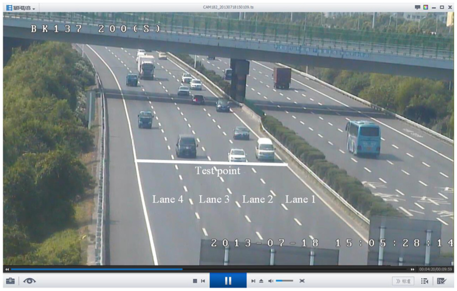
Headway measurement by media software.
There are a total of 36 traffic scenarios of different traffic flow rates, truck percentages, average speeds, and lane positions in the experiment (each scenario for 15 min). Among them, 32 scenarios were used to analyze and determine the best-fitted distribution model for each headway type, and other 4 scenarios were chosen to test the distribution model for each headway type.
Vehicle headway analysis
Preliminary analysis of vehicle headway characteristics
The median value and standard deviation of the vehicle headway were calculated. Table 1 presents the results counted by the lane position and headway type. Since the total vehicle counts in each scenario were for 15 min, the hourly traffic flow rate was obtained by multiplying the vehicle counts by 4.
Median value and standard deviation of the vehicle headway.
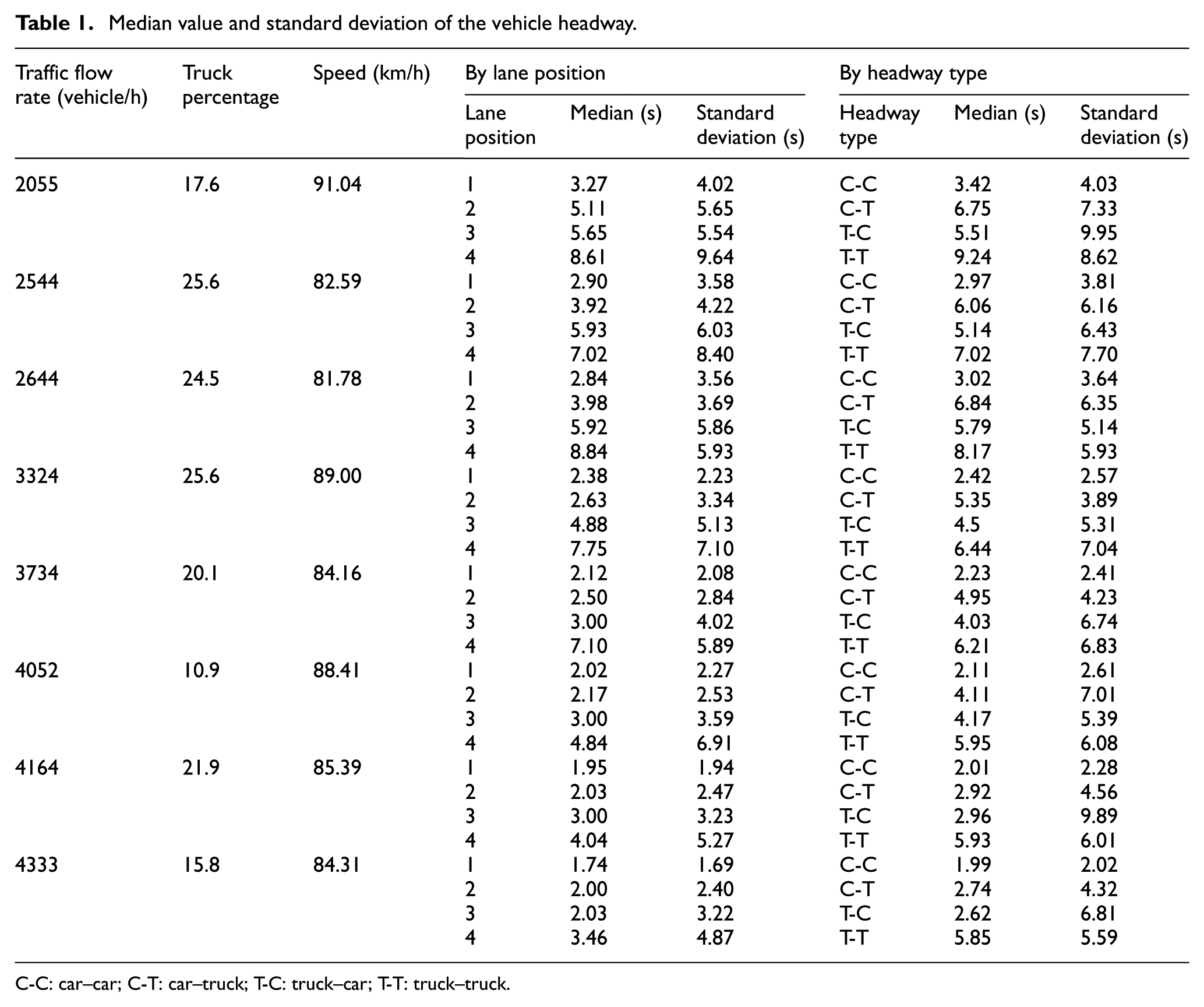
C-C: car–car; C-T: car–truck; T-C: truck–car; T-T: truck–truck.
Among the data shown in Table 1, the median value of the vehicle headway in different lanes decreases with the growth of the traffic flow rate. The range of median headway in lanes 1, 2, 3, and 4 is 1.74–3.27, 2.00–5.11, 2.03–5.93, and 3.46–8.84 s, respectively. Under the same level of the traffic flow rate, the headway in lane 1 is the smallest and the headway in lane 4 is the largest. The headway in lanes 2 and 3 is in the middle range. The standard deviation also has a similar variation trend as the median headway in different lanes. As the lane management is from lane 1 to lane 4, the vehicle composition becomes more heterogeneous, and the performance differences between vehicles become more significant. Therefore, both the value and the discreteness of headway from the inside lane to the outside lane become larger. With regard to the headway by different lead-lag types, the median value becomes smaller as the traffic flow rate becomes higher. Under the same traffic flow rate, the C-C has the smallest median headway, while the T-T has the largest one. When the traffic flow is <4052 vehicle/h, the median values of the C-T are larger than those of the T-C. With the further increase in the traffic flow rate, the median headway of the C-T and T-C is nearly the same. This phenomenon may be due to the different operational characteristics and driving behavior between the truck and the car. The relationship of the standard deviations of the four headway types is little complicated. The standard deviation of the C-C is always the smallest. However, the values for the C-T, T-C, and T-T mix together. The variation trend of the standard deviation of the C-C and T-T is similar, which decreases steadily with the traffic flow rate. Nevertheless, C-T and T-C do not have the obvious trend. A more detailed analysis will be explained in the following section.
Statistical analysis of vehicle headway characteristics
Because the Kruskal–Wallis test and Mann–Whitney U test will have a better effect when the collected headway may not follow the normal distribution, they were used to analyze whether the headway of these four types is different. The results from the Kruskal–Wallis test showed that at a significance level of 0.10, the four headway types were significantly different.
Then, the Mann–Whitney U test was used to test whether any two of the four headway types are also statistically different. The results are shown in Table 2. Except the p value of the C-T and T-C pairs, other results are all <0.10 (two p values of the C-T and T-T are >0.10, but it could be ignored here). So, the C-T and T-C headway types were combined together (represented by C/T), and the Mann–Whitney U test with C-C, C/T, and T-T is used again. It can be seen that all the p values are <0.10 and that C-C, C/T, and T-T are significantly different from each other (as shown in Table 3).
Mann–Whitney U test results for different headway types.

C-C: car–car; C-T: car–truck; T-C: truck–car; T-T: truck–truck.
Traffic flow rate (vehicle/h).
Percentage of truck.
Traffic speed (km/h).
Mann–Whitney U test results for C-C, C/T, and T-T.

C-C: car–car; C/T: C-T and T-C; C-T: car–truck; T-C: truck–car; T-T: truck–truck.
Traffic flow rate (vehicle/h).
Percentage of truck.
Traffic speed (km/h).
Next, the three headway types (C-C, C/T, and T-T) were also analyzed by the Mann–Whitney U test to determine whether they are statistically different when the traffic flow rate, percentage of trucks, and lane position change (traffic speed is highly correlated with traffic flow rate; so, it is excluded here). Table 4 presents the results by different traffic flow rate and percentage of truck, and Table 5 shows the results by different lane positions. The headway for each type is statistically different in both different traffic conditions and different lane positions from the test results of the two tables. Nevertheless, it should be noted that the above non-parametric Kruskal–Wallis test and Mann–Whitney test are univariate statistical techniques which only allow analysis of a single factor at a time. This may give rise to biased results by isolating a single factor for analysis while treating other factors as fixed. In reality, vehicle headway is affected by multiple factors at the same time. Therefore, it is more appropriate to take multiple factors into account simultaneously when describing the vehicle headway distributions. 22
Mann–Whitney U test results by different traffic flow rates and percentages of trucks.
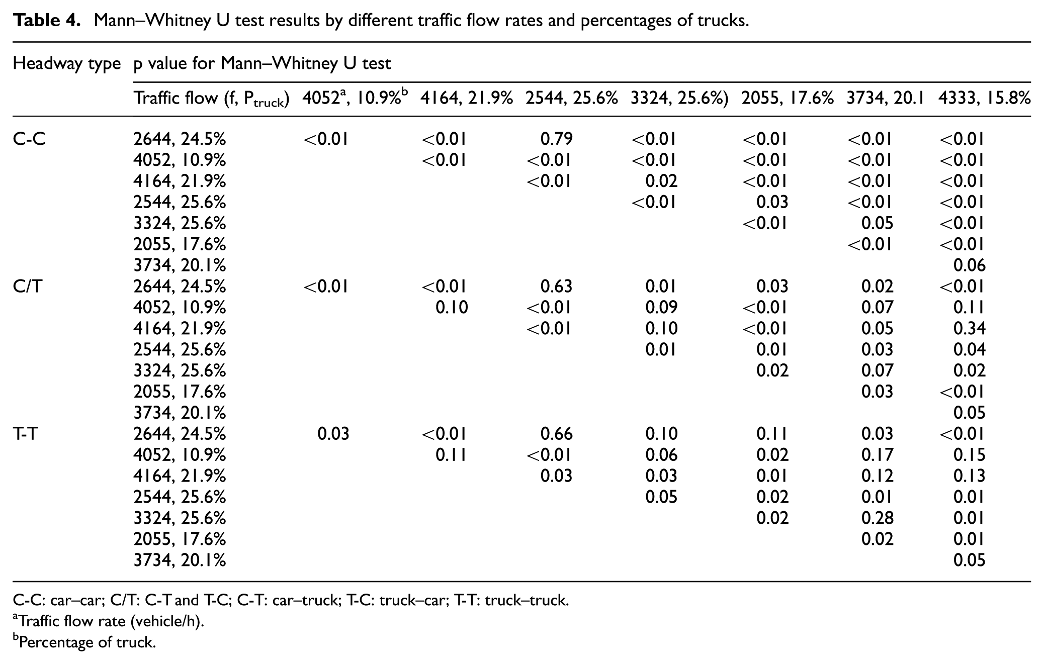
C-C: car–car; C/T: C-T and T-C; C-T: car–truck; T-C: truck–car; T-T: truck–truck.
Traffic flow rate (vehicle/h).
Percentage of truck.
Mann–Whitney U test results by different lane positions.

C-C: car–car; C/T: C-T and T-C; C-T: car–truck; T-C: truck–car; T-T: truck–truck.
There is no C/T and T-T headway types in lane 1.
Vehicle headway distribution
Through the non-parametric tests, C-C, C/T, and T-T headway types are statistically different from each other. In this part, the research will find out the best-fitted distribution model for each particular headway type and will determine the corresponding optimal parameters.
Until now, many researchers have studied the distributions for vehicle headway in different conditions, and some distribution models are most used commonly, such as exponential, Erlang, lognormal, gamma, and normal distribution models. 24 In this study, six candidate distribution models are selected, namely, lognormal, inverse Gaussian, gamma, exponential, normal, and Erlang distributions. The probability density functions are shown as follows:
Lognormal (µ, σ)

Inverse Gaussian (µ, λ)

Gamma (α, β)

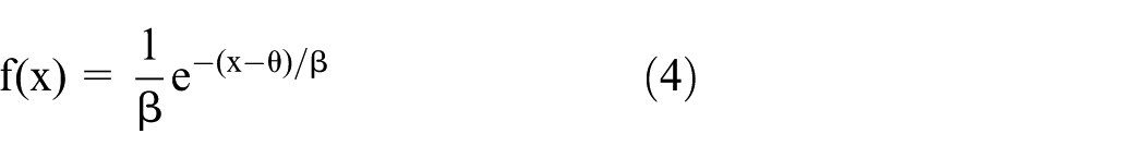
Exponential (β, θ)
Normal (µ, σ)

Erlang (λ, k)

To find out the best distribution model for particular headway type, we will use the considered six distributions to fit the observed headway data for each type under different traffic scenarios (given traffic flow rate, percentage of trucks, and lane position). Then, the K-S tests will be applied to obtain the K-S statistic. During the tests, it should meet the two conditions to be the best-fitted distribution model for a particular headway type under the given traffic scenario. First, the K-S static must be less than the critical value for the K-S test with a level of significance α = 0.05. Second, the K-S static is the smallest among all the six distributions. After determining the fittest distribution model for each headway type under all the traffic scenarios, the distribution model with the most traffic scenarios accepted will become the recommended one for a particular headway type. In the process, @Risk software will be used because it can calculate automatically and quickly to find the consequences.
For example, for the C-C headway type, the traffic scenario is that f = 2644 vehicle/h, Ptruck = 24.5%, and L = 1 (Figure 2). The fitted distribution model according to the @Risk software is listed as follows: lognormal (3.670, 3.206) with K-S static is 0.0840, inverse Gaussian (3.881, 5.975) with K-S static is 0.0846, gamma (1.501, 2.322) with K-S static is 0.1136, exponential (3.462) with K-S static is 0.1628, normal (3.692, 3.557) with K-S static is 0.2065, and Erlang (3.462, 1) with K-S static is 0.1593. As the K-S static of 0.0840 is the smallest among all of them and less than the critical value (0.0876) with a level of significance α = 0.05, the lognormal pattern is the best fitted.

Example of distribution fitting.
Using the method above to look for the best-fitted distribution model pattern for each headway type for all the scenarios, the results are tabulated in Table 6. Lognormal model is the selected distribution model pattern for C-C headway type, which is the best-fitted model in 20 scenarios. In the other 12 scenarios, only 1 scenario rejected the lognormal model because the K-S static is larger than the critical value for the K-S test with a level of significance α = 0.05. Moreover, the K-S static of lognormal model has always been one of the minimum three and the difference between lognormal model and the least one is small. So, the lognormal model could be considered to be the best fitted for overall scenarios. Also, lognormal model is the selected distribution pattern for T-T headway type with 19 scenarios for recommended. There are five scenarios where lognormal model did not fit well, which may be the problem of the samples. For C/T headway type, inverse Gaussian model becomes the selected distribution pattern significantly with 24 scenarios for best fitted. It is accepted in other eight scenarios as well.
Best-fitted distribution patterns for different headway types.

C-C: car–car; C/T: C-T and T-C; C-T: car–truck; T-C: truck–car; T-T: truck–truck.
After the distribution model pattern is determined, the next step is to calculate the parameters. From the lognormal and inverse Gaussian model patterns, we can see that parameters µ and σ determine the specific form of lognormal model and parameters µ and λ determine the specific form of inverse Gaussian model; hence, the functions of (µ, σ) and (µ, λ) should be built. From the previous analysis, it can be seen that the headway varies with the change in traffic flow rates, percentage of trucks, and lane positions. Therefore, (µ, σ) and (µ, λ) can be formulated as functions of these three factors. The maximum-likelihood estimation technique will be used to obtain the functions. The trial-and-error method is used to determine the functional form; the forms with the highest R2 will be finally selected. Table 7 exhibits the final functions of (µ, σ) for lognormal model and (µ, λ) for inverse Gaussian model, and the three coefficients of the variables have significant correlation at the 0.05 significance level.
Functions of (µ, σ) for lognormal model and (µ, λ) for inverse Gaussian model.

C-C: car–car; C/T: C-T and T-C; C-T: car–truck; T-C: truck–car; T-T: truck–truck.
Because of the calibration sample, the parameter functions are valid subject to the following conditions: 2055 vehicle/h ≤ f ≤ 4333 vehicle/h, 10.9% ≤ Ptruck ≤ 25.6%, and L = 1, 2, 3, 4.
For lognormal model, µ represents the mean value and σ2 represents the variance; thus, the mean and standard deviation of the C-C and T-T headway types decrease with the increase in the traffic flow rate and from outside lane to inside lane. It is same as the analysis in section “Preliminary analysis of vehicle headway characteristics.” Also, the mean and standard deviation increase with the percentage of trucks. The intention that drivers like to keep a far distance with trucks to keep a safer driving may cause this trend. Also, it may be related with the range of the traffic condition we set that if the traffic is out of the range, the mean and standard deviation will decrease with the percentage of trucks. For inverse Gaussian model, µ represents the mean value and µ3/λ represents the variance, so the mean of the C/T headway type decreases with the traffic flow rates, the percentage of trucks, and from outside lane to inside lane, but the standard deviation is hard to say.
Model validation
After determining the distribution model pattern and the parameter functions, the performance of the models should be tested. The remaining four observed scenarios, (1) f = 2436 vehicle/h, Ptruck = 25.1%, and L = 3; (2) f = 2032 vehicle/h, Ptruck = 27.0%, and L = 3; (3) f = 3300 vehicle/h, Ptruck = 19.8%, and L = 4; and (4) f = 3678 vehicle/h, Ptruck = 29.2%, and L = 2 (because there is only C-C headway type in lane 1, we did not choose L = 1 as the test sample), are used to evaluate whether the obtained models have a good work.
Depending on the results of the distribution model analysis, the lognormal model is used for C-C and T-T headway types and inverse Gaussian model is used for C/T headway type. Then, using the specific value of the f, Ptruck, and L to calculate the (µ, σ) for lognormal and (µ, λ) for inverse Gaussian, a particular distribution model for the corresponding scenario is obtained. During the model validation, the K-S test and the chi-square test are used to determine the degree of the fitness of the proposed models. If the K-S static and chi-square static are less than the critical value, respectively, with a level of significance α = 0.05, the proposed distribution model will not be rejected. The validation results are shown in Table 8 and Figures 3–5.
Results of validation for the distribution models for a particular headway type.

C-C: car–car; C/T: C-T and T-C; C-T: car–truck; T-C: truck–car; T-T: truck–truck.
Traffic flow rate (vehicle/h).
Percentage of truck.
Lane position.

Lognormal distribution model for C-C headway type: (a) f = 2436 vehicle/h, Ptruck = 25.1%, and L = 3; (b) f = 2032 vehicle/h, Ptruck = 27.0%, and L = 3; (c) f = 3300 vehicle/h, Ptruck = 19.8%, and L = 4; and (d) f = 3678 vehicle/h, Ptruck = 29.2%, and L = 2.

Inverse Gaussian distribution model for C/T headway type: (a) f = 2436 vehicle/h, Ptruck = 25.1%, and L = 3; (b) f = 2032 vehicle/h, Ptruck = 27.0%, and L = 3; (c) f = 3300 vehicle/h, Ptruck = 19.8%, and L = 4; and (d) f = 3678 vehicle/h, Ptruck = 29.2%, and L = 2.

Lognormal distribution model for T-T headway type: (a) f = 2436 vehicle/h, Ptruck = 25.1%, and L = 3; (b) f = 2032 vehicle/h, Ptruck = 27.0%, and L = 3; (c) f = 3300 vehicle/h, Ptruck = 19.8%, and L = 4; and (d) f = 3678 vehicle/h, Ptruck = 29.2%, and L = 2.
From Figures 3–5, comparing input data and proposed distribution models, it is easy to see that the distribution models can describe the particular headway type very well. Also, the results from Table 8 confirm this conclusion through statistical analysis. All the K-S statics and chi-square statics in Table 8 are smaller than the corresponding critical values with 0.05 significance level. The results mean that the proposed distribution models perform well in fitting the observed C-C, C/T, and T-T headways.
Conclusion and discussions
This study was performed to investigate the vehicle headway distribution model at the freeway basic segment under lane management considering car-truck interaction. Through the non-parameter tests (i.e. the Kruskal–Wallis test and Mann–Whitney U test), we found that it is statistically different by the headway type. Thus, the headway was categorized into three types by the leader and follower vehicle types: C-C, C/T (C-T and T-C are not significantly different by the tests, so they are merged together), and T-T. Then, through the Mann–Whitney U test, traffic flow rate, percentage of trucks, and lane position were found having a strong impact on the headway.
To find out the optimal distribution model for each headway type, this study considered six common distribution models (lognormal, inverse Gaussian, gamma, exponential, normal, and Erlang) to fit the C-C, C/T, and T-T headway types. The result is that lognormal model is suitable for C-C and T-T types and inverse Gaussian is accepted by the C/T headway type. Also, we built the parameter functions by traffic flow rate, percentage of trucks, and lane position for a particular distribution model based on the observed 32 traffic scenarios. Then, the remaining four traffic scenarios were used to test the distribution models and parameter functions. The statistical results prove the validity of the proposed models and functions.
This study has developed the distribution models for different headway types and also analyzed the impact of the traffic flow rate, percentage of trucks, and lane position. However, there are some problems need to be studied in the future:
In the actual situation, the traffic flow rate of the freeway can vary from 2000 to 7000 vehicle/h, but in this study, the traffic flow rate is only from 2055 to 4333 vehicle/h. When the traffic flow rate is much higher, the parameter functions may have new forms. Therefore, the range of this study needs to be expanded.
Because of the limitation of conditions, this study only considered six common distribution models to fit the headway types. In the future, more distribution models could be thought to have a test.
There are some differences between the performance of buses and trucks actually in China. In this study, we considered buses and trucks as the same category for convenience. In the future study, the vehicle types can be classified more specifically.
Since the headway has an important impact on car following, lane change, vehicle merge, safety simulation, and evaluation, exploring the characteristics of vehicle headway under lane management considering the car-truck interaction could have a promising help to these areas. In the next step, the findings of this study will be studied to incorporate into the car following, lane change, vehicle merge, safety simulation, and evaluation for better application.
Footnotes
Acknowledgements
The authors would like to thank the colleagues at the School of Transportation at the Southeast University for their assistance in field data collection and data reduction.
Academic Editor: Ling Zheng
Declaration of conflicting interests
The author(s) declared no potential conflicts of interest with respect to the research, authorship, and/or publication of this article.
Funding
The author(s) disclosed receipt of the following financial support for the research, authorship, and/or publication of this article: This research was sponsored by “A Study on Freeway Operation Management Strategy under Saturated Flow” (project no.: 2011-Y-30).