
Abstract
Albeit vehicle analytical models are often favorable for explainable mathematical trends, no analytical model has been developed of the regulated diesel exhaust CO emission rate for trucks yet. This research unprecedentedly develops and validates for trucks a model of the steady speed regulated diesel exhaust CO emission rate analytically. It has been found that the steady speed–based CO exhaust emission rate is based on (1) CO2 dissociation, (2) the water–gas shift reaction, and (3) the incomplete combustion of hydrocarbon. It has been found as well that the steady speed–based CO exhaust emission rate based on CO2 dissociation is considerably less than the rate that is based on the water–gas shift reaction. It has also been found that the steady speed–based CO exhaust emission rate based on the water–gas shift reaction is the dominant source of CO exhaust emission. The study shows that the average percentage of deviation of the steady speed–based simulated results from the corresponding field data is 1.7% for all freeway cycles with 99% coefficient of determination at the confidence level of 95%. This deviation of the simulated results from field data outperforms its counterpart of widely recognized models such as the comprehensive modal emissions model and VT-Micro for all freeway cycles.
Introduction
The rate of regulated exhaust emission is one of the significant vehicle operating costs. 1 Vehicle emission rate modeling is a primary tool for environmentally evaluating the regional impacts of transportation technologies.2,3 Empirical modeling and statistical modeling have been adopted in several research articles in the field of powertrain modeling. 2 For instance, Lindhjem et al. 4 presented the physical emission rate estimator (PERE) which has been developed to complement the MOtor Vehicle Emission Simulator (MOVES) greenhouse gas (GHG) emission model for increasing the level of accuracy in estimating on-road vehicle emissions. They proposed the PERE as an empirical model that is partly based on the principles of physics in order to estimate on-road vehicle emissions. However, the validity of that proposed model is established only for the range of data based on which it was developed. Zito and Doré Landau 5 developed a high-pressure direct injection (HDI) variable geometry turbocharged diesel engine model with variable geometry turbocharger (VGT) and without exhaust gas recirculation (EGR). That model is based on a non-linear black-box identification procedure that is in turn based on a polynomial Nonlinear Auto-Regressive Moving Average with eXogenous inputs (NARMAX) representation for modeling non-linearities. Yet, the model requires recalibration with each dataset. Daw et al. 6 extended an iterated-map model that relates masses of air and fuel, lumped on a cycle basis, with feedback from cycle to cycle via the cylinder residual gases to spark-assisted homogeneous charge compression ignition (HCCI) combustion. This extended model combines diluent-limited flame propagation (spark-ignition (SI)) and temperature-dependent, residual gas driven combustion (HCCI) to compute a combustion extent and integrated heat release for each cycle. Although such mapped model can approximate the global dynamics of the combustion oscillations, it does not employ any chemical-kinetic relations in their solution.
Rakha and Van Aerde 7 developed a microscopic vehicle fuel consumption and emission model called VT-Micro based on instantaneous speed and acceleration. The inputs to the VT-Micro are the instantaneous speed and acceleration and the outputs are instantaneous fuel consumption and emission rates of individual vehicles. Although the VT-Micro model seems to be the leading model in predicting instantaneous emission rates, it is based on empirical formulae and thus provides unexplainable mathematical trends. Rakha et al. 8 pointed out that a widely valid and gear shifting–based microscopic model of diesel engines is sought for evaluating the current/new diesel powertrain technologies.
Empirical and statistical emission models such as MOBILE6 developed by the US Environmental Protection Agency (EPA) attempt to model vehicle emission rate accounting for travel-related factors such as distance and vehicle-related factors such as engine size. 9 However, these models generally fail to capture the effect of roadway-related factors such as road grade and driver-related factors such as driving cycle on vehicle emissions. These models use average speed to estimate vehicle emissions whereas each facility average speed is implicitly based on a driving cycle. Although empirical and statistical models are simple so that they can be easily integrated into vehicle control systems, they are valid only for the range of data based on which they are built.
Vehicle analytical models exhibit several advantages including (1) describing the physical phenomena associated with vehicle operation based on the principles of physical chemistry, (2) providing explainable mathematical trends, and (3) providing extendable modeling to other types of vehicle. However, no analytical model has been developed of diesel engine exhaust CO emission rate yet. 2 The following contributions are accomplished in this article: (1) unprecedentedly developing and validating analytically a model of the steady speed diesel CO exhaust emission rate for trucks (sections “Modeling analytically the steady speed regulated diesel exhaust CO emission rate” and “Validating the developed model experimentally”) and (2) proving through statistical analysis the accomplishment of deviation of 1.7% of the simulated results from the corresponding field data outperforming other widely recognized models such as the comprehensive modal emissions model (CMEM) and VT-Micro for all freeway cycles (section “Statistical analysis of the results of the validation”).
Research idea and methodology
CO2 naturally exists in fresh air. Catalytic converters usually thus convert CO into CO2. In addition, key vehicle emission models such as INTEGRATION do not count CO2 among harmful vehicle emissions. These key models place emphasis on CO when it comes to Cox.10,11 The idea of this article hence is to present and validate an analytical model of regulated diesel exhaust CO emission rate. This study unprecedentedly develops and validates analytically a model of the steady speed diesel CO exhaust emission rate for trucks describing the physical phenomena associated with vehicle operation based on the principles of physical chemistry. The developed model provides explainable mathematical trends and extendable modeling to other types of vehicle. This work is quantitative research based on a theoretical approach employing exploratory and descriptive techniques to analytically model diesel regulated emissions rate. The experimental data for validation have been collected from literature, namely, a previous research work done by our research partner at Virginia Tech based on the Oak Ridge National Laboratory (ORNL) and the US EPA field data. In an endeavor to conduct this research, the following research procedure has been followed:
Conducting literature review in order to substantiate the existence of a research problem;
Establishing an analytical framework and developing an instantaneous, gear shifting–based and microscopic analytical model of CO emission rate;
Conducting simulation based on the devised analytical models using MATLAB;
Carrying out validation through comparison between the results of the simulation of the developed analytical model and the corresponding field data.
The research assumptions in this research include the following assumptions: (1) as to the field data, all vehicles pollute similarly for the same average speed and vehicle-miles traveled; (2) as to the field data, standard deviation in recorded speeds is small so that it can be negligible; (3) the interval variable in the statistical analysis is a random variable that is normally distributed; and (4) the models developed in this study are limited to diesel trucks and light-duty vehicles.
Modeling analytically the steady speed regulated diesel exhaust CO emission rate
The focus of this section is set on the analytical modeling of the rate of the steady speed regulated exhaust CO emission (kg/s),

The analytical models of the
Modeling analytically the steady speed–based CO exhaust emission rate that results from CO2 dissociation
The CO2 dissociation is the first source of CO exhaust emission investigated in this study. The rate of the steady speed–based CO exhaust emissions that result from CO2 dissociation (kg/s),

Given the incompleteness of combustion in diesel engines, the equivalence ratio, Φ, which reflects the influence of the actual concentration of reactants, should appear in the chemical equation of the combustion of diesel fuel. Also, the percentage of burned fuel with respect to total fuel supplied to the cylinder of the engine, that is (1 − RUnburned), should appear in the chemical equation of the combustion of diesel fuel. Thus, equation (3) represents the actual chemical reaction of the combustion of diesel fuel no. 2 in diesel engines following from equation (2)
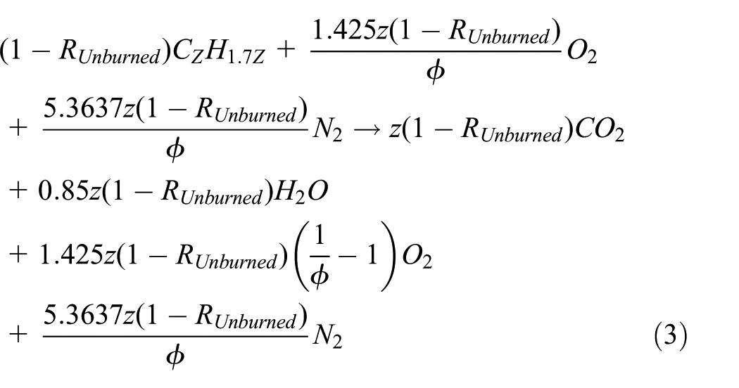
The following chemical reaction therefore describes the CO2 dissociation following from equation (3)

The forward reaction rate at equilibrium based on CO2 dissociation,

Applying the definition of the forward reaction rate at equilibrium based on CO2 dissociation,

The
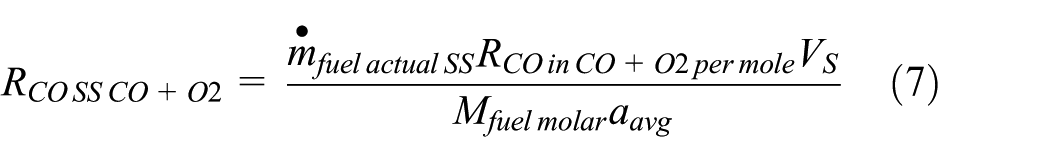
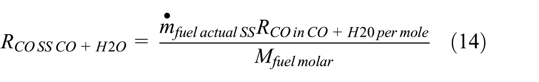
Equation (7) gives in a dimensionally correct form the

The steady speed–based fuel mass flow rate,

The CO2 dissociation is sensitive to high temperature so that the influence of the number of power strokes per mechanical cycle becomes more apparent in CO2 dissociation. The steady speed–based CO exhaust emission rate that results from CO2 dissociation for four-stroke diesel engines (kg/s),
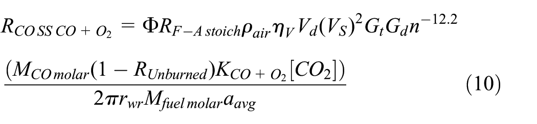
In equation (10), the key explanatory variable is
Modeling analytically the steady speed–based CO exhaust emission rate that results from thewater–gas shift reaction
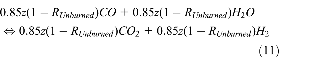
In diesel engines, the chemical reaction of the water–gas shift in the combustion of diesel fuel no. 2 is given following from chemical equation (3) as follows 12
For low-speed cycles, the reverse reaction rate at equilibrium based on the water–gas shift reaction,

Applying the definition of the reverse reaction rate at equilibrium based on the water–gas shift reaction,

The
The

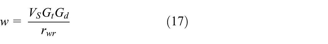
In order to formulate
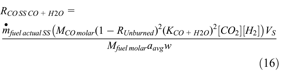
Equation (16) gives
Since the formation of the CO emission is highly sensitive to high temperature, the influence of the number of power strokes per cycle is noticeable on the CO emission rate. In addition, it has been recently found that vehicle speed has an exponential influence on the CO emission rate.
11
Therefore, the steady speed–based CO exhaust emission rate that results from the water–gas shift reaction for low-speed cycles (kg/s),

The steady speed–based CO exhaust emission rate that results from the water–gas shift reaction for high-speed cycles (kg/s),

In equations (18) and (19), the key explanatory variable is
Modeling analytically the steady speed–based CO exhaust emission rate that results from incomplete combustion of HC
The steady speed–based CO exhaust emission rate (kg/s),

The forward reaction rate of incomplete combustion of HC at equilibrium,

Applying the definition of the forward reaction rate at equilibrium based on incomplete combustion of HC,

The

Equation (23) gives in a dimensionally correct form the

The CO formation due to incomplete combustion of HC is sensitive to high temperature so that the influence of the number of power strokes per mechanical cycle becomes more apparent. The steady speed–based CO exhaust emission rate that results from incomplete combustion of HC for four-stroke diesel engines (kg/s),

In equation (25), the key explanatory variable is
Validating the developed model experimentally
In this section, the experimental validation of the developed analytical model is presented for both low-speed cycles and high-speed cycles, respectively. The developed models have been simulated using MATLAB and the simulated results have been validated through comparison with the corresponding field data. The field data were extracted from Rakha et al., 11 West et al., 16 and Brzezinski et al. 17 For the average speed of all the freeway cycles, the field data of the US ORNL and the US EPA are presented. The fact that the measurements presented in the field data are measured by such research authorities in this field further supports the validity of this research. This validation approach further supports the validity of this article in the sense of avoiding bias in measuring the variables under consideration.
The evaluation of
Experimental validation of the developed model of

ORNL: Oak Ridge National Laboratory; EPA: Environmental Protection Agency.
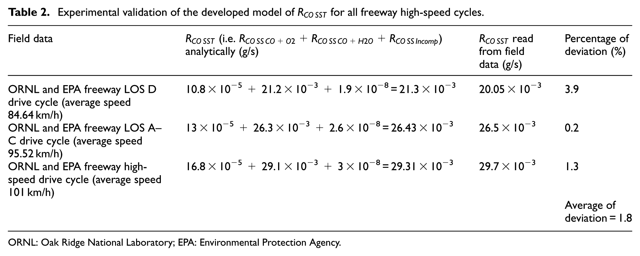
Experimental validation of the developed model of
ORNL: Oak Ridge National Laboratory; EPA: Environmental Protection Agency.
Table 1 gives the validation of the developed models of the
Therefore, the average percentage of deviation between the results of the developed model of

Comparison of the analytical results and field data.
Figure 1 shows the trend of increase in
Statistical analysis of the results of the validation
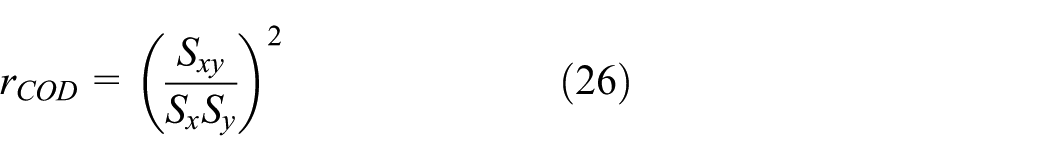
Two measures are used in the statistical analysis of the experimental validation results. The first measure is the coefficient of determination,
The standard deviation of the dataset of the interval variable xi that is the expected value analytically,

Also, the standard deviation of the field dataset of the interval variable yi that is the measured value,

The sample covariance,

The second measure,

Table 3 gives the summary of the statistical analysis of the experimental validation results based on equations (26)–(30).
Summary of the statistical analysis of the experimental validation.

In order to test the significance of this analysis, an inferential statistics-based analysis is conducted in this section. Assuming the interval variable is a random variable that is normally distributed, the following hypothesis is tested comparing the mean of the dataset of the measured values with the set of the analytically expected values


As a matter of fact, the normality assumption is needed to develop the inferential statistical test and moderate departure from normality should not significantly affect the results. 22 The test statistic, tx, is hence evaluated as follows
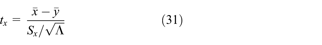
Using Table 3 and for Λ equals to 6, tx is therefore equal to 0.01433. Because we specify the most common value of type I error (α0) of 0.05, the test is two-sided, and both the mean and variance are estimated; then from the t-distribution we find that
Discussion
Modeling diesel exhaust emissions is an effective tool to estimate the rate of vehicle exhaust emissions. The results of the developed models indicated in equations (10), (18), (19), and (25) have been compared with field data and the comparison has indicated good accuracy with
The developed models point out that
The results of this article are supported in the literature. For instance, the three sources of CO formation in internal combustion engines presented in this article are backed as follows: (1) CO2 dissociation,18,12,23 (2) reverse water–gas shift reaction,9,15 and (3) incomplete combustion of HC. 24 In addition, Stephen 24 presented evidence that the first two of the three sources of CO formation in internal combustion engines indicated above are expectedly dominant in comparison with the third one. These three reactions take place simultaneously as can be gathered from Stephen 24 that shows in the first couple of chapters of the book that the normalized fractions of combustion species based on CO2 deposition are 3.6 × 10⁻⁴ for CO and 0.9994 for CO2 at 1500 K and 1 atm. In addition, Stephen 24 shows in the first couple of chapters of the book that the normalized fractions of combustion species based on the water–gas shift reaction are 0.12 for CO and 0.88 for CO2 at 2268 K and 1 atm. It is noteworthy that once the exhaust valve of the cylinder is opened, the pressure of the exhaust gases drops instantaneously to the level of the atmospheric pressure. It is also noteworthy that the water–gas shift reaction is exothermic in the direction of the formation of CO which further helps the formation of CO by providing further heat to favor the formation of CO.
In real engines, the H2O is traces. In addition, the majority of the H2O traces is consumed in the water–gas shift reaction since the water–gas shift is the dominant reaction in carbon oxide formation. The majority of the remaining of the traces of H2O combines with the unburned fuel to form CO. The incomplete combustion of HC as a source of CO has been further taken into consideration in this research in terms of (1 − Runburned), that is, the percentage of burned fuel. In techniques such as “steam reforming” that are sometimes used in power engineering in applications such as fuel cells, H2O is added purposely so that its percentage is notable whereas the scope of this article is limited to typically standard diesel engines. In addition, the water–gas shift reaction is a two-way chemical reaction and both ways of reaction take place in internal combustion engines. For instance, Stephen 24 shows that the normalized fractions of combustion species based on the water–gas shift reaction are 0.12 for CO and 0.88 for CO2 at 2268 K and 1 atm. The incomplete combustion of HC has been analytically modeled by the authors in another article. 25
The developed model addresses a moment after opening the exhaust valve in the exhaust system at the average temperature of exhaust. The developed model does not need to incorporate an additional section of “after-treatment” for several reasons: (1) the developed model predicts the CO formation rather than CO2 formation, (2) there is no analytic conversion to convert CO2 into CO, and (3) there is no catalytic converter to convert CO into CO2 but through the water–gas shift reaction which is included in the developed model.
For decades, there has been an ever-growing list of regulatory standards on diesel fuel to address concerns about the environment. A key cause of excessive harmful exhaust emission is improper dispersion of fuel in the combustion chamber of the engine due to incorrect viscosity of the diesel fuel used. Emission estimation techniques help in assessing how efficient diesel fuels are produced and how efficient diesel engines are designed for reducing emissions in compliance with regulatory standards for reduced harmful impact on the environment, particularly in the developed countries such as United States and Europe. Appendix 8 highlights key regulatory standards on automotive diesel fuel.
The results presented in this study are limited to trucks and light-duty vehicles. The developed analytical models can help in cost-effectively estimating the actual rate of exhaust emission rate for the environmentally sustainable development of diesel powertrain technologies. These models quantify a significant source of air pollution that negatively affects the atmosphere helping in evaluating the relative risks associated therewith. The developed models can serve applications such as the INTEGRATION microscopic traffic simulator.
Conclusion
The diesel steady speed emission rate of CO as a key harmful pollutant has been analytically modeled in this article. Among the backing facts that support the validity of the developed models is that the models have been developed following from the principles of physical chemistry. Another backing fact is that these models are dimensionally correct. For all freeway cycles, the simulated results indicated in equations (10), (18), (19), and (25) have been compared with field data and the comparison has shown with
Footnotes
Appendix 1
Appendix 2
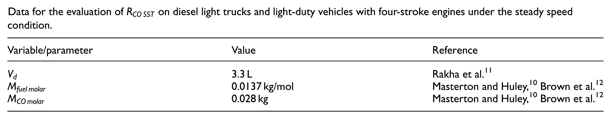
Data for the evaluation of

| Variable/parameter | Value | Reference |
|---|---|---|
| Equivalence ratio, | 0.7 | Guensler et al. 14 |
| Air density at the outlet of the supercharging compressor, | 1.7 kg/m3 | Guensler et al. 14 |
| Volumetric efficiency, | 0.9 | Kane 28 |
| Displaced volume, | 0.00033 m3/d-cycle | Guensler et al. 14 |
| Vehicle tire rolling radius, | 0.323 m | Guensler et al. 14 |
| Stoichiometric fuel–air ratio | 0.0696 | Heywood 18 |
| Gear ratio at the engine transmission, , and the gear ratio in the final drive, , for freeway LOS G cycle (vehicle average speed of 20.96 km/h) | Gt of 1.43 and Gd of 2.5 | Rakha et al., 11 West et al., 16 Brzezinski et al. 17 |
| Gear ratio at the engine transmission, , and the gear ratio in the final drive, , for freeway LOS F cycle (vehicle average speed of 29.76 km/h) | Gt of 1.43 and Gd of 2.5 | Rakha et al., 11 West et al., 16 Brzezinski et al. 17 |
| Gear ratio at the engine transmission, , and the gear ratio in the final drive, , for freeway LOS E cycle (vehicle average speed of 48.8 km/h) | Gt of 1 and Gd of 2.5 | Rakha et al., 11 West et al., 16 Brzezinski et al. 17 |
| Gear ratio at the engine transmission, , and the gear ratio in the final drive, , for freeway LOS D cycle (vehicle average speed of 84.64 km/h) | Gt of 1 and Gd of 2.5 | Rakha et al., 11 West et al., 16 Brzezinski et al. 17 |
| Gear ratio at the engine transmission, , and the gear ratio in the final drive, , for freeway LOS A–C cycle (vehicle average speed of 95.52 km/h) | Gt of 1 and Gd of 2.5 | Rakha et al., 11 West et al., 16 Brzezinski et al. 17 |
| Gear ratio at the engine transmission, , and the gear ratio in the final drive, , for freeway high-speed cycle (vehicle average speed of 101 km/h) | Gt of 1 and Gd of 2.5 | Rakha et al., 11 West et al., 16 Brzezinski et al. 17 |
Appendix 3
Data for the evaluation of

| Variable/parameter | Value | Reference |
|---|---|---|
| Equivalence ratio, | 0.7 | Guensler et al. 14 |
| Number of moles of diesel fuel no. 2 in the reactants per unit mass of working fluid, | 1 | Rakha et al., 11 West et al., 16 Brzezinski et al. 17 and Heywood 18 |
| Standard enthalpy of formation of diesel fuel no. 2 in the reactants per unit mass of working fluid (in J/M) at ambient temperature, , since the dominating largest portion of reactants enters the cylinder of the engine at quasi-ambient conditions | 454.5 × 10³ J/M | Rakha et al., 11 West et al., 16 Brzezinski et al. 17 and Heywood 18 |
| Number of moles of O2 in the reactants per unit mass of working fluid, | 22.8 | Rakha et al., 11 West et al., 16 Brzezinski et al. 17 and Heywood 18 |
| Standard enthalpy of formation of O2 in the reactants per unit mass of working fluid (in J/M) at ambient temperature, , is 0 J/M; the number of moles of N2 in the reactants per unit mass of working fluid, | 85.82 | Rakha et al., 11 West et al., 16 Brzezinski et al. 17 and Heywood 18 |
| Standard enthalpy of formation of N2 in the reactants per unit mass of working fluid (in J/M) at ambient temperature, | 0 J/M | Rakha et al., 11 West et al., 16 Brzezinski et al. 17 and Heywood 18 |
| Number of moles of CO2 in the products per unit mass of working fluid, | 16 | Rakha et al., 11 West et al., 16 Brzezinski et al. 17 and Heywood 18 |
| Standard enthalpy of formation of CO2 in the products per unit mass of working fluid (in J/M) at ambient temperature, , since the pressure drop in the exhaust occurs instantaneously when the exhaust valve opens and the exhaust pressure then becomes atmospheric | 393.5 × 10³ J/M | Rakha et al., 11 West et al., 16 Brzezinski et al. 17 and Heywood 18 |
| Number of moles of H2O in the products per unit mass of working fluid, | 13.6 | Rakha et al., 11 West et al., 16 Brzezinski et al. 17 and Heywood 18 |
| Standard enthalpy of formation of H2O in the products per unit mass of working fluid (in J/M) at ambient temperature, | 241.8 × 10³ J/M | Rakha et al., 11 West et al., 16 Brzezinski et al. 17 and Heywood 18 |
| Number of moles of N2 in the products per unit mass of working fluid, | 85.82 | Rakha et al., 11 West et al., 16 Brzezinski et al. 17 and Heywood 18 |
| Standard enthalpy of formation of N2 in the products per unit mass of working fluid (in J/M) at ambient temperature, | 0 J/M | Rakha et al., 11 West et al., 16 Brzezinski et al. 17 and Heywood 18 |
Appendix 4
Appendix 5

Appendix 6
Data for the evaluation of

Appendix 7
Data for the evaluation of

| Variable/parameter | Value | Reference |
|---|---|---|
| 2.7 × 10⁻¹⁴/mol2/s | Flagan and Seinfeld 27 | |
| 1 M | Masterton and Huley, 10 Brown et al. 12 | |
| Z | 16 for n-hexadecane (C16H34) which is the most widely used type of fuel oil no. 2 that is a heavier distillate than fuel oil no. 1 with hydrocarbons in the C11–C20 range | US Agency for Toxic Substances and Disease Registry 26 |
| 1 M | Masterton and Huley, 10 Brown et al. 12 | |
| 0.504 M | Masterton and Huley, 10 Brown et al. 12 | |
| 0.504 M | Masterton and Huley, 10 Brown et al. 12 |
Appendix 8
Acknowledgements
The technical support provided by the Faculty of Engineering at the International Islamic University Malaysia (IIUM) as well as by the Center for Sustainable Mobility at Virginia Polytechnic Institute and State University (Virginia Tech) is thankfully acknowledged.
Academic Editor: Jose Ramon Serrano
Declaration of conflicting interests
The author(s) declared no potential conflicts of interest with respect to the research, authorship, and/or publication of this article.
Funding
The author(s) disclosed receipt of the following financial support for the research, authorship, and/or publication of this article: This study was financially supported by the IIUM under research grant # RMGS 09-10 and also by the Center for Sustainable Mobility at Virginia Tech under the research project “TranLIVE UTC - U.S. Department of Transportation”.