Sage Journals: Discover world-class research

Abstract

The acoustic signals of internal combustion engines contain valuable information about the condition of engines. These signals can be used to detect incipient faults in engines. However, these signals are complex and composed of a faulty component and other noise signals of background. As such, engine conditions’ characteristics are difficult to extract through wavelet transformation and acoustic emission techniques. In this study, an instantaneous frequency analysis method was proposed. A new time–frequency model was constructed using a fixed amplitude and a variable cycle sine function to fit adjacent points gradually from a time domain signal. The instantaneous frequency corresponds to single value at any time. This study also introduced instantaneous frequency calculation on the basis of an inverse trigonometric fitting method at any time. The mean value of all local maximum values was then considered to identify the engine condition automatically. Results revealed that the mean of local maximum values under faulty conditions differs from the normal mean. An experiment case was also conducted to illustrate the availability of the proposed method. Using the proposed time–frequency model, we can identify engine condition and determine abnormal sound produced by faulty engines.

Keywords

Instantaneous frequency engine abnormal sound faulty time–frequency

Introduction

Engines are important apparatuses in most machineries, which work at high speeds and heavy loads under severe environmental conditions.¹ When engines become faulty, fault diagnosis systems should promptly distinguish the engine conditions of fault engines to prevent engine deterioration and to ensure proper machinery functioning for a long period. Faulty mechanical systems are often diagnosed on the basis of acoustic and vibration signals that contain large data regarding the operating parameters and physical conditions of engines.^2–4 However, existing methods can distinguish the faulty type of engines but cannot achieve the target of real-time online diagnosis. In engineering practice, experienced technicians hear abnormal sounds when engines are in faulty conditions.^5–7 Our study aims to confirm whether a fault diagnosis system can automatically identify engine conditions and whether engines remain functional under faulty. Several methods are used to detect engine or machine conditions. Tan and colleagues^8–10 investigated unsteady flows in a centrifugal pump volute under non-cavitation and cavitation conditions using a computation fluid dynamics framework. The main methods of engine fault diagnosis based on sound signals include wavelet transform and mode decomposition.^11–13 Similar to Fourier transformation technology, wavelet transformation technology can provide information regarding frequency domain, some characteristics can be extracted in the frequency domain.^5,14–16 Shirazi and Mahjoob¹⁷ diagnosed the condition of a four-cylinder internal combustion (IC) engine using discrete wavelet transform to decompose vibration signals and to obtain appropriate wavelet layers. Nevertheless, fault diagnosis in wavelet transformation is complex, and the characteristic frequency should be initially extracted. Wavelet function also varies in different faults. Mode decomposition has been proposed by Huang, and his colleagues proposed and used empirical mode decomposition (EMD); in this process, any complicated signal can be decomposed into a collection of intrinsic mode functions based on local timescale characteristics of the signal.¹⁸ Yadav and Kalra¹⁹ decomposed an engine signal through EMD and applied a feature technique to diagnose an IC engine. Despite these advantages, wavelet transformation and mode decomposition based on sound/vibration signal analysis exhibit several weaknesses.²⁰ Wavelet transformation results highly depend on the ability of the selected wavelet basis function to yield high coefficients, while all other features are masked or completely ignored.²¹ EMD mainly depends on experience and is associated with several problems, such as end effect and mode confusion. Although this field has been extensively investigated, an efficient method that can resolve EMD-related problems has yet to be established. In some instances, faults in engines are determined, but fault type is not identified. This chapter focuses on identifying whether an engine is good or defective. Therefore, an instantaneous frequency technique was proposed.

Instantaneous frequency technique

Engines experience two types of fault. The first type occurs when two or more parts of an engine scrape one another. The other type ensues when an engine is exposed to shock. Figure 1 illustrates a typical shocking acoustic signal with an acute change at the starting point. Most shocking acoustic signals exhibit the same features.

Figure 1.

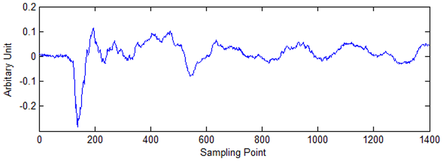
Example of a shocking acoustic signal.

A faulty component is possibly large when an abnormal sound is produced; otherwise, abnormal sounds may be masked by background noise when a faulty component signal is small. The relationship between the maximum value ratio of pure shocking signal to background noise and hearing clarity degree is shown in Figure 2. The ration was obtained through a hearing experimentation in Coolpro software. When the hearing clarity degree reaches 40%, abnormal sound can be heard obviously.

Figure 2.

Relationship between the maximum value ratio of pure shocking signal to background noise and hearing clarity degree.

Differences in function can be described as the change rate. The acute change position can be acquired; therefore, the differential value at the moment when an abnormal sound is produced is larger than that obtained at other moments. However, the background exhibits randomness, and large values may be present. As such, the difference function cannot be used to identify engine conditions. Therefore, the instantaneous frequency technique was proposed to solve this problem.

The instantaneous frequency technique was derived from a simple inverse triangle algorithm; in this algorithm, a unique frequency value can be obtained at any time. In this method, the instantaneous frequency can be extracted from a time domain model, which was then used as the basis for the construction of a new time–frequency model.

A fixed amplitude (amplitude = 3) and a variable frequency sine function were used to fit a pair of adjacent points gradually (Figure 3). The sine function frequency of the two points can be determined as the frequency of the former point. One frequency is detected at one point.

Figure 3.

Schematic of adjacent points fitting.

Two adjacent sampling points, namely, X and Y, whose values are x and y, are used. The fitting function is sin(wp+q). w and q can be calculated using the known x and y in the fitting function

{\begin{matrix} x = \sin (w p_{1} + q) \\ y = \sin (w p_{2} + q) \end{matrix}

(1)

where x is value of point X, y is value of point Y, w is frequency of point X, q is phase of point X, and p₁ and p₂ are a pair of adjacent given sampling points.

Inverse sine transformation is applied to equation (1)

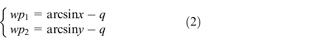
{\begin{matrix} w p_{1} = \arcsin x - q \\ w p_{2} = \arcsin y - q \end{matrix}

(2)

where p₂ − p₁ = 1; w, which can be expressed in equation (3), can be calculated using equation (2)

w = \arcsin x - \arcsin y

(3)

w can be substituted into Equation (2) and the phase q can be calculated as follows

q = \arcsin x - w p_{1}

(4)

We can use this method to calculate the instantaneous frequency at any time (at any sampling point). The instantaneous frequency is single value which is related to other points.

No negative values are found in the frequency domain; therefore, w should be considered as an absolute value

{\tilde{w}}_{i} = | w_{i} | = | \arcsin x_{i + 1} - \arcsin x_{i} | where i = 1, 2, \dots, n

(5)

The parameter ${\tilde{w}}_{i}$ is the frequency of the sampling point, and the real frequency is defined as follows

{\tilde{w}}_{ri} = \frac{{\tilde{w}}_{i}}{fs} where i = 1, 2, \dots, n; f_{s} is the sampling rate

(6)

The acoustic signal of the faulty engine (F_n) is composed of background noise (F_bn) and malfunction sound (F_mn)

F_{n} = F_{bn} + F_{mn} n = 1, 2, 3, \dots

(7)

where n is sampling point.

The acoustic signal is F_bn when the engine is in good condition. However, the acoustic signal is F_n when the engine malfunctions; extremely high F_n is even detected. Consequently, the instantaneous frequency range of the high extreme point and the time–frequency model change; thus, the engine condition can be detected.

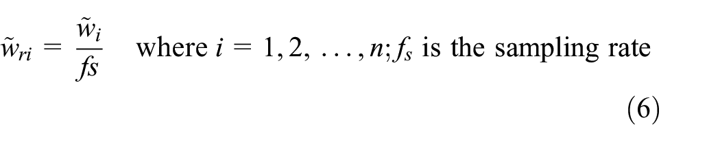
The instantaneous frequency value between two adjacent sampling points is relative to the signal intensity. Therefore, the two time–frequency models of two signals which have the same waveform and the different signal intensity are different. A normalization method was proposed to solve the above problem. The calculation process is described as follows:

Find the global maximum value from time–frequency model

{\tilde{w}}_{max g} = max ({\tilde{w}}_{ri}) where i = 1, 2, \dots, n

(8)

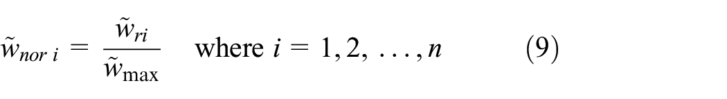
Normalize the time–frequency model

{\tilde{w}}_{nor i} = \frac{{\tilde{w}}_{ri}}{{\tilde{w}}_{max}} where i = 1, 2, \dots, n

(9)

In this study, a simply auto-identification of engine conditions was proposed. The process of this method is described as follows:

Find all local maximum value points from the time–frequency model

\begin{matrix} {\tilde{w}}_{max lj} = l max ({\tilde{w}}_{i}) where {\tilde{w}}_{i} > {\tilde{w}}_{i - 1} \\ and {\tilde{w}}_{i} > {\tilde{w}}_{i + 1}, i = 1, 2, \dots, n, \\ j = 1, 2, \dots, m \end{matrix}

(10)

Calculate the mean value of all local maximum values

{\tilde{w}}_{mean} = \sum_{1}^{n} {\tilde{w}}_{max lj} where j = 1, 2, \dots, m

(11)

The value at the moment an abnormal sound signal occurs is larger than that at other moment. Therefore, the mean of all local maximum values of the abnormal sound signal is higher than mean of all local maximum values of the normal sound signal in the normalized time–frequency model. The computer automatically detects the abnormal sound when the mean decreases.

The following section describes the advantage of the instantaneous frequency technique over the difference method. We defined S_s as the shocking component, S_g as the background noise, and S_c as the mixed signal, where S_c = S_s + S_g and the maximum value of S_s is greater than that of S_g. The difference function of S_c can be denoted as $S_{c}^{'} = S_{c} (n + 1) - S_{c} (n)$ , where n is a sampling point. The instantaneous frequency function of S_c can be denoted as ω = |arcsin[S_c(n+1)] − arcsin[(S_c(n))]|. The relationship between ω and the values of two adjacent points is shown in Figure 4(a). Figure 4(b) illustrates $S_{c}^{'}$ .

Figure 4.

Value range of (a) ω and (b) $S_{c}^{'}$ and (c) comparison.

Figure 4 shows that ω is larger than S_c when the sampling points are the same. As the sampling point value increases, the increase in ω is higher than that of $S_{c}^{'}$ . Figure 2 illustrates that the maximum value of a shocking component is larger than that of the background at the same time. Therefore, ω at the moment an abnormal sound occurs is larger than that at other moments.

Simulated experiment

A simulated experiment was conducted to verify the validity of the time–frequency domain method. The test data of background noise are acquired from a serve motor. The fault data are generated using an aluminum wire to scratch the bulge of a roundel mounted on the output end of the motor (Figure 5).

Figure 5.

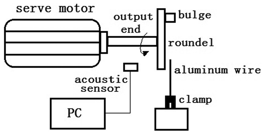
Simulated experimental apparatus.

The sound signal comprises the sound of a running serve motor and a scratching sound, which is an aliasing signal (Figure 6(b)). The signal without a scratched sound is shown in Figure 6(a). The sampling rate of the acoustic sensor is 44,100. When the serve motor is running at an operating speed of 180 r/min, the aluminum wire periodically scratches the bulge mounted on the rim of the roundel, and the acoustic sensor collects the sound signal in real time. The data of the normal sound and the scratching sound are then processed in a personal computer and the corresponding time–frequency model (Figure 6(c) and (d)) is established. The moment of scratching is distinguishable from other moments (Figure 6(d)) because the value is larger than that obtained at other moments, which is indicated by red circles. The normalized time–frequency models of the normal signal and the scratched signal are shown in Figure 6(e) and (f). The normalized frequency can be used to create a statistical model and to identify whether an abnormal sound is produced.

Figure 6.

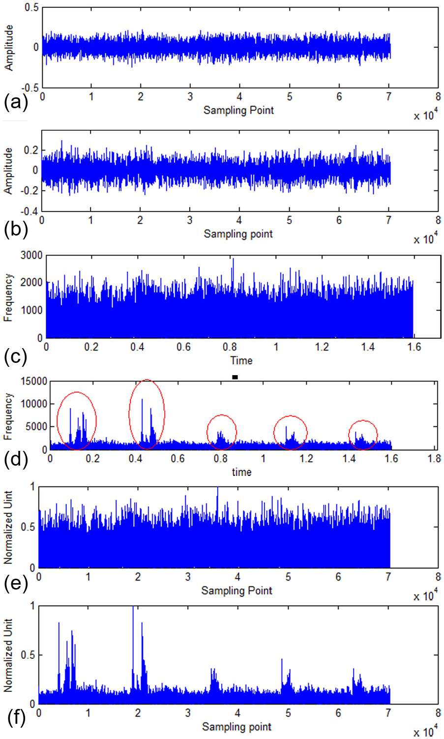
Original signal, time–frequency model, and normalized time–frequency model of non-scratching and scratching sound signals: (a) non-scratching sound signal, (b) scratching sound signal, (c) time–frequency model of non-scratching sound signal, (d) time–frequency model of scratching sound signal, (e) normalized time–frequency model of non-scratching sound signal, and (f) normalized time–frequency model of scratching sound signal.

The means of a non-scratching sound signal and a scratching sound signal in the normalized time–frequency model are expressed as follows

\begin{matrix} {\tilde{w}}_{mean normal signal} = 0.2966 \\ {\tilde{w}}_{mean scratched signal} = 0.0917 \end{matrix}

On the basis of two parameters, we can distinguish the scratching sound signal from the non-scratching signal.

Experiment

Experiments were conducted in a 34-kW four-stroke three-cylinder gasoline engine using a Sennheiser E945 acoustic sensor placed on the outer engine block (Figure 7). Table 1 lists the engine specifications and Table 2 lists the sensor parameters.

Figure 7.

Experimental apparatus.

Table 1.

Engine specification.

Engine type	BYD371QA
Bore stroke	84.00 mm
Displacement	998.00 mL
Compression ratio	10.50:1
Charged method	Naturally aspirated

Table 2.

Sensor parameters.

Sensor type	Sennheiser E945
Frequency response range	40–18,000 Hz
Sensitivity (free field)	(1 kHz) 2.0 mV/Pa
Normal impedance	350 Ohm
Minimum end impedance	1000 Ohm

Data were acquired from the gasoline engine (BYD371QA) when one of the cylinder bores marked with a red-cross was scuffing. The experiments were performed at a speed of 800 ± 30 and 1800 ± 30 r/min. The acoustic sound was detected by the sensors, whose sampling frequency was 44,100 Hz. Two acoustic sensors were used in case one sensor interfered with the other components, but only one group of data was chosen. The normal sound data were obtained from the same engine after this engine was repaired. The original signal should be filtered by a low pass filter whose threshold is 2000 Hz to eliminate the high-frequency interference.

The normal signal and the scuffing cylinder bore signal with a speed of 800 ± 30 r/min are shown in Figure 8(a) and (b). The two signals did not evidently differ. The corresponding time–frequency models are shown in Figure 8(c) and (d). However, the faulty engine of one model could not be distinguished from the other model. When listening to the sound signal with a speed of 800 ± 30 r/min, we could not also identify the faulty signal between the normal signal and the scuffing cylinder bore signal.

Figure 8.

Original signal and time–frequency model of a normal cylinder and a scuffing cylinder at a speed of 800 ± 30 r/min: (a) normal signal at an engine speed of 800 ± 30 r/min, (b) scuffing cylinder bore signal at an engine speed of 800 ± 30 r/min, (c) time–frequency models of the normal signal at an engine speed of 800 ± 30 r/min, and (d) time–frequency models of the scuffing cylinder bore signal at an engine speed of 800 ± 30 r/min.

The normal signal and the scuffing cylinder bore signal at a speed of 1800 ± 30 r/min are shown in Figure 9(a) and (b), respectively. These signals did not remarkably differ from each other. However, the normal model was different from the scuffing cylinder bore model in the terms of time–frequency domain (Figure 9(c) and (d)). In the time–frequency model of the normal signal, no abnormal change was detected. By contrast, the maximum values were high (marked with red circles) in the time–frequency model of the scuffing cylinder bore signal. A clicking sound indicating a faulty sound signal could be heard by human ears, and the moment of the clicking sound is matched with the maximum value in the time–frequency model of the scuffing cylinder bore through listening.

Figure 9.

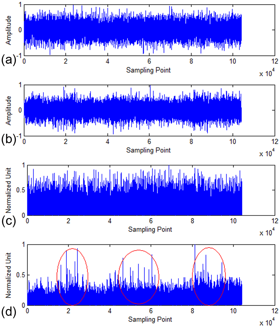
Original signal and time–frequency model of a normal cylinder and a scuffing cylinder at a speed of 1800 ± 30 r/min: (a) normal signal at an engine speed of 1800 ± 30 r/min, (b) scuffing cylinder bore signal, (c) normalized time–frequency model of a normal signal, and (d) normalized time–frequency model of a scuffing cylinder bore signal.

The means of the normal sound signal and the scuffing sound signal in the normalized time–frequency model are expressed as follows

\begin{matrix} {\tilde{w}}_{mean normal} = 0.2612 \\ {\tilde{w}}_{mean scuffing} = 0.1137 \end{matrix}

The faulty condition indicated by the corresponding signal can be easily identified because ${\tilde{w}}_{mean normal}$ is much bigger than ${\tilde{w}}_{mean scuffing}$ .

The results of the proposed method and the wavelet transform method are compared in Figure 10. The original signal originated from the scuffing cylinder at a speed of 1800 ± 30 r/min (Figure 9(b)). The wavelet transform method was applied to perform a four-layer db10 wavelet decomposition. To facilitate the comparison, we transformed the wavelet layers into the same form; the absolute values were calculated and then normalized. The d3 wavelet layer (Figure 10) is similar to the normalized time–frequency model (Figure 9(d)). However, appropriate wavelet function and wavelet layer should be selected in practical applications.

Figure 10.

Comparison of wavelet transform and inverse trigonometric instantaneous frequency analysis methods.

Another experiment was performed to examine the bolt looseness fault in an engine bonnet. The original signal and the normalized time–frequency model (Figure 11) were described in this study. Figure 11 illustrates that the normalized time–frequency model can identify the looseness fault. Therefore, the method proposed in this study can be applied widely.

Figure 11.

Original signal and normalized time–frequency model of the bolt looseness fault in an engine bonnet.

Conclusion

This study presented a new time–frequency model of faulty diagnosis. The proposed model was verified through a simulated experiment and a series of field experiments by applying different speeds in a simple test-bed and a running three-cylinder engine. The main conclusions are as follows:

The new time–frequency model was proposed in the article, the calculating process was introduced, and the method was verified through a series of experiments.

The method was based on abnormal sounds that could be identified by human ears. The abnormal sound can be distinguished easily by the time–frequency model when an engine produces a regular abnormal sound. By contrast, the faulty condition of the engine can be hardly identified when the engine produces a slightly regular abnormal sound or an irregular abnormal sound.

Footnotes

Academic Editor: Teen-Hang Meen

Declaration of conflicting interests

The author(s) declared no potential conflicts of interest with respect to the research, authorship, and/or publication of this article.

Funding

The author(s) disclosed receipt of the following financial support for the research, authorship, and/or publication of this article: This work was financially supported by the Fundamental Research Funds for the Central Universities (No. 3132015091), Liaoning Natural Science Foundation (No. 2014025007), National Key Technology Support Program (Nos 2014BAB12B05 and 2014BAB12B06), National Natural Science Fund (No. 51275063), and Dalian science and technology planning project (2014A11GX023).

References

Gao

Duan

Fan

. Rotating machine fault diagnosis using empirical mode decomposition. Mech Syst Signal Pr 2008; 22: 1072–1081.

Rezaei

Dadouche

Wickramasinghe

. A comparison study between acoustic sensors for bearing fault detection under different speed and load using a variety of signal processing techniques. Tribol Lubr Technol 2014; 70: 77–86.

Anami

Pagi

VB.

Acoustic signal-based approach for fault detection in motorcycles using chaincode of the pseudospectrum and dynamic time warping classifier. IET Intell Transp Sy 2014; 8: 21–27.

Mba

Rao

RBKN

. Development of acoustic emission technology for condition monitoring and diagnosis of rotating machines: bearings, pumps, gearboxes, engines, and rotating structures. Shock Vib Digest 2006; 38: 3–16.

Czech

Wojnar

Burdzik

. Application of the discrete wavelet transform and probabilistic neural networks in IC engine fault diagnostics. J Vibroeng 2014; 16: 1619–1639.

Kim

Jang

JW.

A study on development of engine fault diagnostic system. Math Probl Eng 2015; 2015: Article ID 271374 (6 pp.).

Moosavian

Najafi

Ghobadian

. Piston scuffing fault and its identification in an IC engine by vibration analysis. Appl Acoust 2016; 102: 40–48.

Tan

Zhu

Wang

. Numerical study on characteristics of unsteady flow in a centrifugal pump volute at partial load condition. Eng Computation 2015; 32: 1549–1566.

Yuchuan

Lei

Baoshan

. Numerical investigation of influence of inlet guide vanes on unsteady flow in a centrifugal pump. P I Mech Eng C: J Mec 2015; 229: 3405–3416.

10.

Lei

Shan

Liang

. Numerical simulation of unsteady cavitation flow in a centrifugal pump at off-design conditions. P I Mech Eng C: J Mec 2014; 228: 1994–2006.

11.

Van

Kang

HJ.

Two-stage feature selection for bearing fault diagnosis based on dual-tree complex wavelet transform and empirical mode decomposition. P I Mech Eng C: J Mec 2016; 230: 291–302.

12.

Xiong

Pan

HP.

A method of discriminating fault against oscillation based on empirical mode decomposition. Dynam Cont Dis Ser A 2006; 13: 83–87.

13.

Lei

Lin

. A review on empirical mode decomposition in fault diagnosis of rotating machinery. Mech Syst Signal Pr 2013; 35: 108–126.

14.

Wang

Liu

. Fault diagnosis of diesel engine based on adaptive wavelet packets and EEMD-fractal dimension. Mech Syst Signal Pr 2013; 41: 581–597.

15.

Liu

Zhang

TH.

Fault diagnosis for micro-gas turbine engine sensors via wavelet entropy. Sensors 2011; 11: 9928–9941.

16.

Liu

CH.

Investigation of engine fault diagnosis using discrete wavelet transform and neural network. Expert Syst Appl 2008; 35: 1200–1213.

17.

Shirazi

Mahjoob

. Application of discrete wavelet transform (DWT) in combustion failure detection of IC engines. In: Proceedings of the 5th international symposium on image and signal processing and analysis, Istanbul, 27–29 September 2007, pp.482–486. New York: IEEE.

18.

Huang

Shen

Long

. The empirical mode decomposition and the Hilbert spectrum for nonlinear and non-stationary time series analysis. P Roy Soc A: Math Phy 1998; 454: 903–995.

19.

Yadav

Kalra

. Fault diagnosis of internal combustion engine using empirical mode decomposition. In: Proceedings of the 6th international symposium on image and signal processing and analysis (ISPA 2009), Salzburg, 16–18 September 2009, pp.40–46. New York: IEEE.

20.

Robertson

Park

Alvin

KF.

Extraction of impulse response data via wavelet transform for structural system identification. J Vib Acoust 1998; 120: 252–260.

21.

Fernandes

FCA

van Spaendonck

RLC

Burrus

CS.

Multidimensional, mapping-based complex wavelet transforms. IEEE T Image Process 2005; 14: 110–124.