Sage Journals: Discover world-class research

Abstract

In this article, the principles of programming in the Sleptsov net language are further developed with respect to the restrictions on the control flow and its composition with data. The conditions of correctness of Sleptsov net programs are formulated in the form of additional restrictions on copying parameters of modules and using global variables. Flags are added for correct manipulation by shared data. In the general case without restrictions on the program composition rules, the problem is reduced to the soundness of workflow nets with shared resources; there are several useful particular cases when the algorithm complexity is polynomial. Examples of Sleptsov net programs for the fast solution of production control tasks are presented.

Keywords

Petri net Sleptsov net programming control flow shared resources

Introduction

Model driven software development is a fundamental current approach for developing software. In the case of general purpose software, the Unified Modeling Language (UML)¹ has received a lot of attention, also for the development of security-critical software.^2,3 For specialized classes of software, alternative (e.g. domain-specific) approaches can be more appropriate, for instance in the case of software for production automation and especially programmable logic controllers.⁴ For programmable logic controllers, the application of the Petri net (PN) programming language has considerable advantages (such as an expressive graphical language, formal methods to prove correctness, and the ability to support concurrent programming).⁵ Usually, a PN processor is implemented as a software interpreter of PN behavior which launches usual routines which load transitions, arcs, and tokens of PNs. In spite of the advantages mentioned above, a wide application of PN languages has been hampered because the implementations of basic arithmetic operations within PNs have exponential time complexity. Thus, in practical implementations, PNs have been combined with the use of programming languages. This in turn makes the working environment inhomogeneous, which creates obstacles for a seamlessly integrated application of formal methods for model-checking the PN models and a hardware implementation of PN processors.

In Zaitsev,⁶ a more general class of Sleptsov nets (SNs) was introduced and studied from a computational point of view, which opens many possibilities for efficient concurrent computations implemented using the uniform approach of SN programming. Programs written in high-level SNs are compiled into a low-level plain SN and executed on an SN hardware processor. The Universal SN^7,8 is a prototype of such a processor. The approach provides hyper-performance as explained in Zaitsev⁶ where examples of its application to control systems, based on partial differential equations and fuzzy logic, are considered.

In this article, we work out the principles of SN program composition which is defined in Zaitsev.^6,9 In particular, we present a technique for an efficient correctness proof of SN programs. The current work mainly targets the application area of logical controllers and automated control. Future work will deal with the integration of the approach within a general purpose software development tool, and the development of data types needed in that context.

An overview of SN programming

An SN is a bipartite directed multi-graph supplied with a dynamic process.⁶ An SN is denoted as $N = (P, T, W, μ_{0})$ , which includes the following:

P and T are disjoint sets of vertices called places (drawn as circles) and transitions (drawn as rectangles), respectively.

The mapping W specifies arcs between vertices.

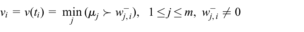
$μ_{0}$ represents the initial state (marking).

The mapping $W : (P \times T) \to N \cup {- 1}, (T \times P) \to N$ defines the types and multiplicities of arcs, where:

A zero value corresponds to the absence of an arc.

A positive value corresponds to the regular arc with indicated multiplicity.

A negative value corresponds to the inhibitor arc which checks whether a place contains an empty marking.

Here $N$ denotes the set of natural numbers. To avoid nested indices we denote $w_{j, i}^{-} = w (p_{j}, t_{i})$ and $w_{i, j}^{+} = w (t_{i}, p_{j})$ .

The mapping $μ : P \to N$ is used to specify the place marking. To determine the multiplicity of firability conditions on each incoming arc of a transition, the following auxiliary operation is defined

x ≻ y = {\begin{matrix} x / y, & if y > 0 \\ 0, & if y = - 1, x > 0 \\ \infty, & if y = - 1, x = 0 \end{matrix}

To avoid inconsistency arising from an infinite number of instances, we disallow transitions without regular incoming arcs. The dynamic behavior of an SN is represented as the result of applying the following transition firing rule:

The number of instances of a transition $t_{i}$ firable at the current step is equal to

v_{i} = v (t_{i}) = \min_{j} (μ_{j} ≻ w_{j, i}^{-}), 1 \leq j \leq m, w_{j, i}^{-} \neq 0

When a transition $t_{i}, v_{i} > 0$ fires, for $u_{i} \leq v_{i}$ the following is carried out:

$u_{i} \cdot w_{j, i}^{-}$ tokens are extracted from each input place $p_{j}$ for regular arcs $w_{j, i}^{-} > 0$ of the transition;

$u_{i} \cdot w_{i, k}^{+}$ tokens are placed onto each of output places $p_{k}$ , $w_{i, k}^{+} > 0$ of the transition.

The net halts if firable transitions are absent.

For concurrent implementations, we allow several firable transitions to fire at a given step of execution.

In a PN, only one transition fires at a given execution step in one instance ( $u_{i} = 1$ ). This situation can be obtained as a particular case of an SN attaching (via self-loop) to each transition a place with a marking equal to 1. Thus, an SN subsumes all the advantages of a PN, while it improves the concept of a PN by providing an efficient implementation of basic arithmetic operations in polynomial time (as demonstrated in Zaitsev⁶), whereas these operations require exponential time in a PN.

The principles of programming in the PN language are presented in a refined form in Zaitsev.⁹ Here, a program is represented as a composition of a control flow (CF) with data stored in PN places. In this context, the concept of a module having input and output places was introduced. Its execution is controlled via a pair of dedicated CF places: the input place Start (S) launches the module while the output place Finish (F) indicates its completion. Initially, input and internal places of a module are required to be empty. Before the module is launched, its input parameters are copied from the relevant places into its input places. After a module finishes its execution, its output parameters are assigned to the corresponding places. To simplify the parameter assignment process, the notation of copying arcs was introduced. Dashed and dotted arcs connect a module with the places that store the variables and represent the subnets CLEAN, MOVE, COPY, and their combinations.

High-level nets (which are represented by a hierarchy of modules) are compiled into a plain inhibitor PN for the execution on a PN processor (implemented either in software or in hardware). This compilation process consists of the substitution of modules in an in-line or call-return fashion and the expansion of dashed/dotted arcs by the subnets assigning the variables in a sequential or concurrent way.

Standard patterns of the CF composition have been introduced in the above-mentioned publication (such as sequencing, branching, looping, paralleling of subnets), while the CF is not restricted to these patterns. A CF connects an obligatory place Start with another obligatory place Finish. All the CF places are initially empty. Putting a token into the place Start launches the program, and the arrival of a token at the place Finish indicates the completion of the program. At the program completion, all other CF places are supposed to be empty.

As mentioned above, SNs allow an efficient implementation of arithmetic operations (in particular multiplication and division) in polynomial time. In Zaitsev,⁶ it was shown that SNs run with a high level of performance, and the peculiarities of programming in SNs were studied, which include standard CF patterns, modules for basic arithmetic and logic operations, and the principles of compiling them into low-level plain nets.

As an important property, SNs use a reverse CF represented by moving zero markings. Using a straight CF with moving tokens (units) checked via regular arcs having unit multiplicity restricts the number of firable instances of a transition to the unit. Using the reverse CF with moving zero markings (checked via an inhibitor arc) does not restrict the number of firable instances of a transition at a step, which allows us to demonstrate the advantages of SNs for the efficient implementation of operations.

As discussed in Zaitsev,^6,9 the advantages of this approach are achieved to a maximal degree using hardware PN or SN processors with a massively parallel implementation of the transition firing process. Small universal nets^7,8 represent preliminary prototypes of such processors, while the best prototypes should employ a concurrent firing of transitions.

In current work, we use an ad-hoc software simulator of SNs to execute them, which accepts a net specification in the form of a sparse incidence matrix. An SN processor as a plug-in for the system Tina¹⁰ will allow using Tina as a graphical editor for SNs. Moreover, the possibility to integrate the SN firing rules into future versions of the Tina system has been discussed with the system developers. This will allow using its stepper simulator for debugging SN programs and its reachability tree tools for proving correctness of SN programs.

Properties of the CF of SN programs

In the previous papers on the PN Programming Language and SNs,^6,9 no explicit restrictions were put on the composition of the CF. Here, we consider three classes of CF: an unrestricted CF, a reverse conveyor workflow net (WFN),⁹ and a composition of standard patterns. In the context of unrestricted CF, some useful subclasses can be separated from potentially dangerous structures. In particular, a WFN¹¹ requires that each node lays on a route from the Start place S to the Finish place F. A WFN represents a well-studied class of PNs. In particular, it can be shown that a closed WFN is live and bounded. The corresponding property is called soundness (more specifically, 1-soundness when a single token is put into the net as assumed for WFNs). Sometimes, the connections used need to be more restricted in order not to distract conveyor processes (as shown in Figure 1). Note here that the reverse CF pattern (c) corresponds via an injective mapping to the straight conveyer structure pattern (b). For such nets, we can also study k-soundness by substituting the Start place by a chain of k places. For the three scenarios in Figure 1(a)–(c), the same (unique) execution sequence is valid when assuming that the starting place contains a single token; the difference consists in the corresponding sequence of markings:

For Figure 1(a) and (b), it is (1, 0, 0, 0), t₁, (0, 1, 0, 0), t₂, (0, 0, 1, 0), t₃, (0, 0, 0, 1).

For Figure 1(a), it is (0, 1, 1, 1), t₁, (1, 0, 1, 1), t₂, (1, 1, 0, 1), t₃, (1, 1, 1, 0).

Figure 1.

Types of control flow: (a) straight, (b) straight conveyor, and (c) reversed (conveyor).

The difference between Figure 1(a) and (b) can be seen in the case of initial markings greater than 1. Basic constructs for the Sleptsov net control flow (SNCF) composition (as shown in Figure 2), are as follows:

Single action (transition).

Par-begin-end.

Branching.

Loop (while).

Figure 2.

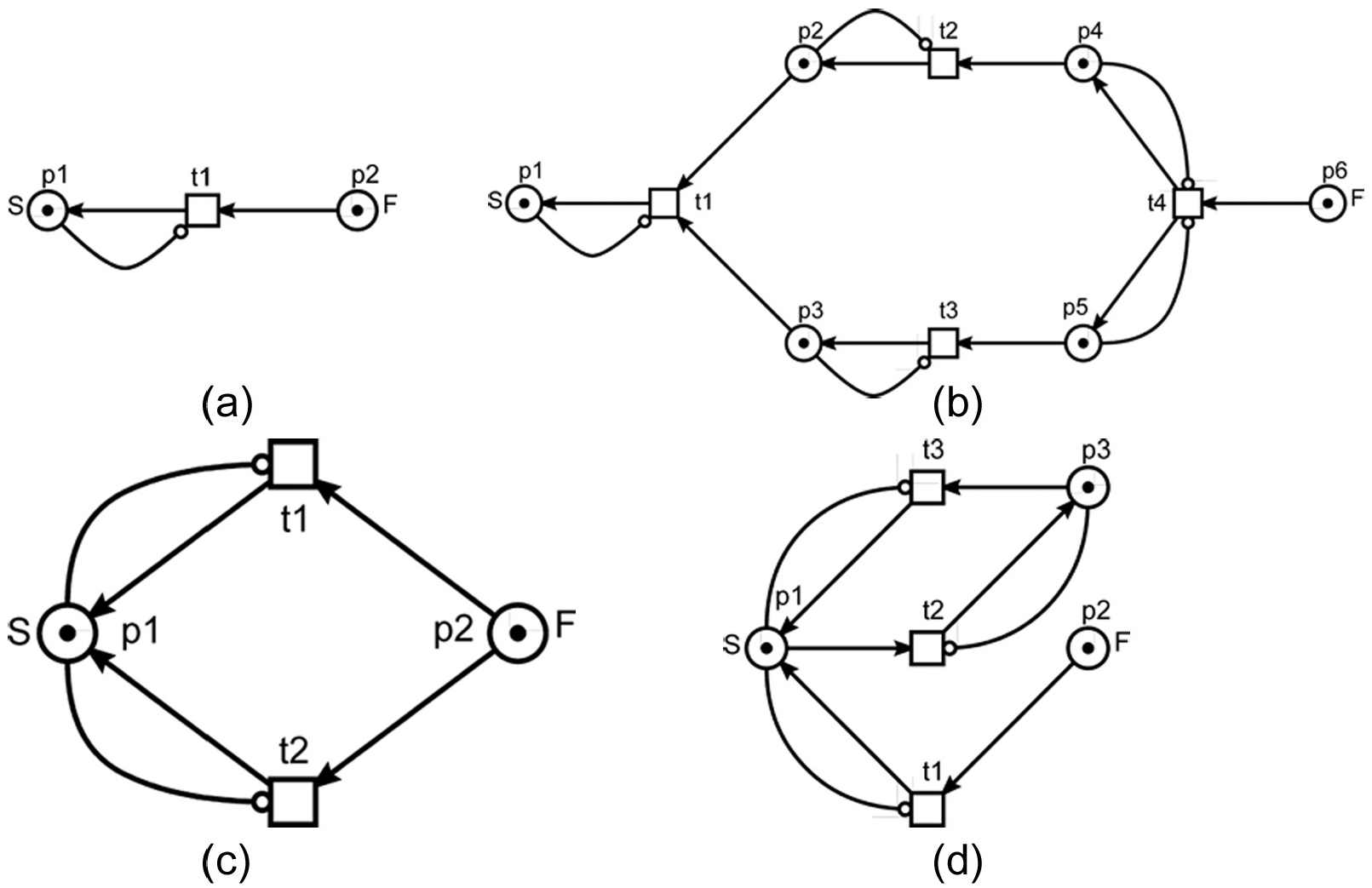
Basic CF constructs: (a) single action, (b) parallel processes, (c) branching (alternative processes), and (d) loop.

Note that Figure 2 does not include additional nodes which restrict branching and loops (for instance, logical variables calculated by some modules). Usually, the loop condition is recalculated during the execution of the loop. In examples of real-life programs (cf. for instance Figure 8), these variables can be represented by dedicated PN places.

For the nets shown in Figures 2 –4, all the places contain a token in the initial marking which is specific to the reverse CF. Because of the inhibitor arcs that are present, none of the transitions is firable and each net stands still. To launch it, we need to remove a token from the start place (S). This enables the corresponding transition, and then the moving zero marking represents the CF. Note that in the majority of the examples seen here, some places have duplicate identifiers (such as the character “p” followed by a number, and in addition individual names for the most significant of them, such “S” and “F”).

Figure 3.

Sequential composition.

Figure 4.

Substitution.

To compose a strict CF using the Sleptsov net programming language (SNPL), we suggest the following composition rules:

Sequential composition (Figure 3). Merging the Finish place F of previous with the Start place S of the next.

Substitution (Figure 4). Replacing a single transition of a construct with another construct; for example, the transition t₂ in Figure 3 by a Loop construct.

In many cases, we first need to substitute a transition by a sequence of transitions and then to substitute one of the transitions by a subnet: for instance, to use the first transition for checking a condition and the second for the concrete computations implementing this condition. We close SNCF in the way also usual for WFNs: by adding a transition connecting F with S (Figure 5).

Figure 5.

Closing CF.

Statement 1

Any closed strict SNCF is a live and bounded net.

Proof

First, each of the basic CF constructs shown in Figure 2 is a live and bounded net which transforms its initial marking S = 0 into its final marking F = 0. Second, each of the composition rules creates a live and bounded net from live and bounded components which transform their initial marking S = 0 into their final marking F = 0.

Lemma 1

Any SNCF is isomorphic to a WFN with a single token.

Proof

First, there is structural isomorphism of one-to-one correspondence for places and transitions. As for arcs, in an SNCF we simply replace:

Each arc that connects a place with a transition by an arc of a reverse direction.

Each arc that connects a transition with a place together with corresponding inhibitor arc, by a single arc of reverse direction.

To obtain the initial marking, we remove the tokens from all marked places and put a token into the place S. In a similar way, we can specify a mapping of WFNs into SNCF. For a single token, a transition is firable in the source net if and only if it is firable in the transformed net (which is a WFN). For the resulting markings of two nets, the following inverting mapping is valid: $1 \leftrightarrow 0$ , $0 \leftrightarrow 1$ .

For weak rules of composition, we require that each node lays on a regular arcs route from F to S.

Theorem 1

Any closed SNCF is a live and bounded (1-bounded) net.

The proof immediately follows from Lemma 1 and the soundness of WFNs.¹¹ For similar results regarding k-soundness, we can attach a “speed-up strip” of k places and transitions with k zeros to the SNCF.

In the next section, we now consider strict rules of SNPL composition which correspond to structural parallel programming (compared to previous work,⁶ smaller patterns are specified and more restricted composition rules are used).

Concurrent data access rules

From section “Properties of the CF of SN programs,” we can conclude that a CF subnet in an SN program is a correct structure which is a live and bounded net. Attaching data to a CF net (either directly or by making use of modules) can include deadlocks and overflows. We now study these issues in detail. As for the best known results on deadlock avoidance, the state-of-art paper¹² represents the front edge of modern research providing a maximally permissive control.

A module includes input, output, and internal places. In the most restricted form, it represents a functional subnet (a so-called clan). For brevity, we allow incoming regular arcs from the module transitions for input places. Among input places, there is one dedicated CF place—Start (S), and among output places there is one dedicated CF place—Finish (F). Moreover, we divide the internal places of a module into CF places and places which store variables.

When a module only uses its input, output, and (local) variables’ places, we call it a closed module. Closed modules are a restricted kind of module, and thus programming using closed modules only facilitates proving the correctness of programs. When several modules can use the same variable’s place, they are called open modules and the corresponding variable is called a global variable.

In case the modification of global data is implemented using transitions whose execution is interleaved with the execution of other transitions, each global variable used in more than one path from F to S should be supplied with an access flag (semaphore).

Besides CF transitions, modules employ transitions which modify data (input/output or internal (global) variables). Usually, the execution of such transitions is controlled by the CF places, namely by inhibitor arcs connecting a place to a transition. Thus, a transition which modifies data only fires when the corresponding CF place is equal to zero. These kinds of connections are illustrated in Figure 6 (where the net has been launched with the removal of token from the place $p_{1}$ ).

Figure 6.

Interaction of CF with other nodes.

In addition to this, the execution of the CF can be controlled by data places. This increases the complexity of the interconnections between CF and data, and thus complicates the correctness proof of the program. By assuming that the module behaves correctly under certain conditions, we can identify conditions for the correctness of the entire program which is composed of modules that satisfy these assumptions.

Closed modules only

When using only closed modules, one can prove the program correctness under the assumption that the module behavior is correct (which means that it finishes within a number of steps bounded by the upper bound of its time complexity and produces a correct result). We further assume a correct combination of input data. In Figure 7, a scheme for accessing variables using flags is shown. For each variable v_i, there is an access flag gv_i. Before accessing a variable, it is seized by a transition (for instance, seize-v1-vn for v₁–v_n) and after finishing access to a variable, it is released by a transition (for instance, release-v1-vn for v₁–v_n). Of the CF places (at the bottom of the figure), the starting place (S) does not contain a token (which corresponds to the launched state of the net where the leftmost transition is firable).

Figure 7.

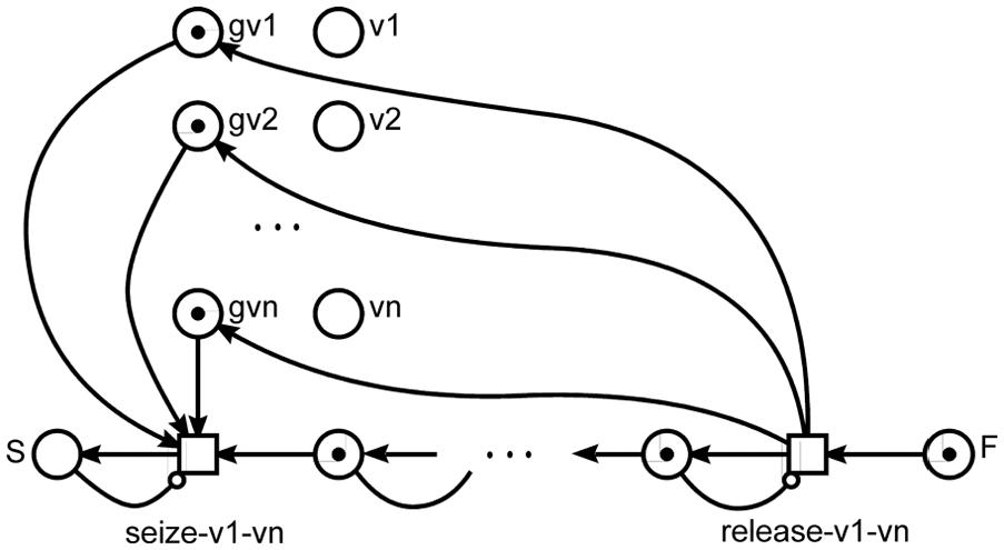
Flags for access to variables.

Without restriction of generality, we consider two levels of hierarchy in the following. For an arbitrary number of levels, we can extend the following proof by use of induction. Under the assumption that modules work correctly, the only threat to the program correctness can arise from moving data to/from input/output places, respectively, by dashed and dotted arcs.

Statement 2

If a variable’s place is employed in a single path from S to F, then it is used correctly when it is copied to/from only one input/output place of each module.

Proof

A single path represents a sequential order of actions which are not executed concurrently for the variable (i.e. the next action uses the variable after the previous one). Thus, there is no simultaneous modification of the variable value.□

The statement could be strengthened by considering alternative sequential paths only. In that case only one of them is active at a given point in time, so no other module/transition concurs for the variable place.

For each other variable’s place, we attach a flag place with zero marking in order to check availability of the variable using an inhibitor arc. We will control the execution of each assignment action by setting a flag before the execution of the action and resetting the flag after its execution. For an example of using an addition module,⁶ the use of variables is shown in Figure 8. Two variables a and b are seized by the transition seize-a-b; then they are copied by two COPY modules into the input places of the module ADD. After ADD has finished, the variable c is seized by the transition seize-c. The variable c is cleaned by CLEAN module and then the result is moved from the ADD module output place z to the place c. Finally, the variable c is released by the transition release-c. All of the CF places except S contain a token, which satisfies the requirements of the reverse CF. The absence of a token in the starting place S corresponds to the initial state of the net.

Figure 8.

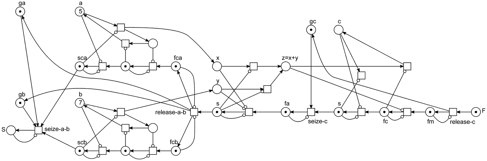
Data access control example (c = a + b).

Theorem 2

In case a program net with dashed arcs does not contain deadlocks and each module uses a variable as an input only once, copying variables via the procedure using flags described above does not cause any deadlocks (i.e. the net after expansion of dashed arcs and attaching flags is deadlock-free).

Proof

First, the copying, cleaning, and moving modules that are substituted in place of the dashed arcs are deadlock-free, as well as the entire net. Second, before the execution is started, the corresponding variable is locked and after the execution is finished, the corresponding variable is unlocked. Moreover, there are no variables seized in sequence.

Theorem 3

When a module uses the same variable as an input several times, there are no deadlocks in the following cases:

Using a global variable as an input variable in the same module for an unlimited number of times (seizing and releasing it individually for each dashed arc).

Each global variable used as an input variable in the same module several times is copied using the modified parallel copying module shown in Figure 9.

Figure 9.

Multiple copying module (y1 = x, y2 = x,…, yn = x).

Proof

The first item is proven as a corollary of Theorem 2, because only one dashed arc at its extension sets the corresponding flag and all the actions are executed in sequence; the same applies to the sequential copying technique.⁹ The proof of the second item is based on the correctness of extensions for a single target variable⁶ and the fact that a transition $t_{1}$ splits the value of the variable x simultaneously into all places y1, y2,…, yn. Thus, there is no competition for the place of the variable x.□

Note that the initial marking in Figure 9 corresponds to the launched parallel copying of the value 45 from the place x to the places y1–yn. We now consider the source of deadlocks in SNPL with closed modules: besides a CF subnet, we use variable places, variable flag places, and data modifying transitions. Data modifying transitions, local variable places attached to the CF, and data copying subnets pose a threat to the correctness of SNPL programs.

Basic set of elementary modules for the composition of correct and efficient programs

Let us eliminate non-CF transitions and places from all modules (except elementary ones whose correctness is already proven). The goal of correctness and efficiency should not lead to restricting the set of recursive functions too far. In the context, efficiency means to allow no slow-down compared to the computation of a Turing Machine (especially in computing basic arithmetic and logic functions). In fact, we limit the time complexity of basic operations such as addition, subtraction, multiplication, and division–modulo.

The following set of SNPL modules provides an efficient and correct implementation of basic arithmetic and logic operations:

ADD—addition.

SUB—subtraction.

MUL—multiplication.

DIV—division and modulo.

GT—comparison.

NOT—negation.

OR—disjunction.

AND—conjunction.

And the following set of modules extends dashed arcs:

CLEAN—cleaning.

COPY—copying variable value.

MOVE—moving variable value.

For the modules mentioned above, the correctness proof is presented in Zaitsev,⁶ where their time complexity is also estimated. The time complexity is comparable to Turing machines and exponentially faster than for PNs.

Thus, we conclude that programming in SN produces correct programs when using basic modules and the composition rules described in section “Properties of the CF of SN programs.” The only threat appears when composing data and control flow. In initial CF net patterns, branching and loop structures can also be represented in a way which can be abstractly described as a nondeterministic choice. When composed with data which controls the branching of loops, live-locks can appear (as common for sequential programming languages as well^1,2). Note that live-locks can lead to data overflow (i.e. unbounded nets).

Correctness of open modules

Open modules give more freedom when working with data, but they contain the potential treat of deadlocks. To mitigate this risk, there are two possible schemes for accessing global variables:

Seize all variables at once when entering a module and release them when leaving it.

Seize a variable when we start modifying it and release it when finish modifying.

Theorem 4

When SN program accesses external variables only according to the scheme (1), it contains no deadlocks.

Proof

First, all the variables which are required for the module work are seized simultaneously using a single transition (i.e. there is no sequential seizing of resources). The proof is finished using the assumption that each module terminates in finite time and live-locks are absent.

Some notes on deadlock avoidance techniques

After a reasonable restriction of the SNPL programming technique, we can conclude that a restricted SNPL net represents a deadlock-free concurrent program. Deadlocks are possible when using the data modifying transitions in arbitrary way inside modules, and also in case of the scheme (2) discussed above when global variables can be seized/released sequentially. Note that the usual threat of live-locks appears after the net extension when working with given data.

For the unrestricted schemes mentioned above, there is an isomorphism to the problem for WF with resources.¹³ The corresponding algorithm for finding deadlocks and for enforcing liveness was studied in Bashkin and Lomazova,¹⁴ and Sidorova.¹⁵ In spite of the fact that it is nondeterministic polynomial-time hard (NP-hard) in the general case,¹⁶ there are several useful particular cases when the algorithm complexity is polynomial (for instance, for one unbounded resource¹⁴ and for conservative nets¹⁷).

Examples of SN programs

First, we study an example which reveals benefits of the technique developed in this article compared to the direct encoding of algorithms by SNs.⁶ Then we solve a classical task of control specifying a transfer function by an SN. Alternative approaches^18–20 are based on hybrid and colored PNs which use discrete, continuous, and timed transitions as well as special functions to distinguish and transform tokens. Benefits of hybrid and colored PNs consist in their expressive power which leads to laconic constructs. However, minimalism of SN concept, which is obtained only via an extension of the PN transition firing rule with multiple firing, constitutes it advantage.

Multiplication using a compositional approach

Compared to Zaitsev⁶ we compose a multiplication module not directly but by assembling it out of the modules CLEAN, ADD, M2, DM2, for which correctness is already shown. The result is shown in Figure 10; subnets are represented as transitions with a double border. The motivation is that, first, it is simpler and, second, it has the same polynomial complexity.

Figure 10.

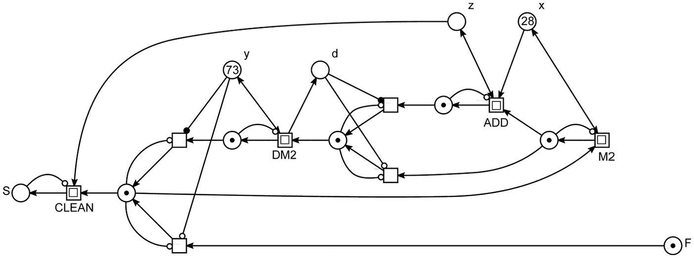
Multiplication composed in a modular way.

Subnets M2 and DM2 implement multiplication by 2 and division–modulo by 2, respectively. The initial marking of the net shown in Figure 10 corresponds to the launched multiplication for x = 28 by y = 73.

Fast solving production control tasks by SNs

Many tasks within production control can be specified using fuzzy logic.^21,22 All stages of a typical controller execution can be programmed efficiently using SN: fuzzification, defuzzification, and the rule base. An example of an SN computing a fuzzy logic function (which could be considered as a way of rules specification) is studied in Zaitsev.⁶ Moreover, the publication⁶ presents an example for fast numerical solving of Laplace equations. Complex tasks of control can be specified using partial differential equations such as Laplace equations, which has many applications for example in thermodynamic processes, electric chains control, and so on. The difference schemes for solving such equations numerically are the source data for their fast implementation using SNs.

Various problems of production control, described with (partial) differential equations,²³ can be reduced to the calculation of the corresponding transfer function²⁴ (which represents a polynomial or a quotient of polynomial, or their sum). In many publications, the required control is obtained via hybrid PNs or other kinds of PN extensions^{18–20,25,26} which use some external facilities for the efficient computation of algebraic expressions. At any rate, computations implemented via PNs are inefficient. Within the domain of manufacturing systems, models from this domain are often combined with PN models, which leads to heterogeneous tools and hampers formal verification and the integration of analysis tools.

The application of SNs provides an efficient computation of transfer functions for many typical controlled processes. An output of a linear system with a transfer function $G (s)$ is described as $y (t) = G (s) u (t)$ or $y = Gu$ , where $u (t)$ is an input and $y (t)$ is an output.

For instance, consider the following transfer functions²⁷ which specify the stated functions:

$G (s) = ks$ , Bode plot of a differentiator.

$G (s) = \frac{k}{s}$ , Bode plot of an integrator.

$G (s) = \frac{a}{s + a}$ , Bode plot of a first order system.

$G (s) = a^{2} / (s^{2} + 2 a ζ s + a^{2})$ , Bode plot of a second order system.

$G (s) = (10 {(s + 1)}^{2}) / s$ , Bode plot of an ideal proportional–integral–derivative (PID) controller.

Note that the Bode plot of either an integrator or diffentiator is computed using a single SN transition. For the calculation of the Bode plot of other systems, efficient division/multiplication SN modules such as the ones considered above are employed.

A special case of the discrete-time general state space model is the linear state space model²⁸ specified by the following system

{\begin{matrix} x (k + 1) = A x (k) + B u (k) \\ y (k) = C x (k) + D y (k) \end{matrix}

where $x (k)$ represents the system state at time step (tact) k, A is the transition matrix, B is the input matrix, C is the output matrix, and D is the direct output matrix; in most cases $D = 0$ . For provisioned matrices, the corresponding SN uses their components’ values as the constant multiplicity of arcs, which provides a very efficient re-computation of the state and output implemented with SN shown in Figure 11 (which uses the direct data flow control).

Figure 11.

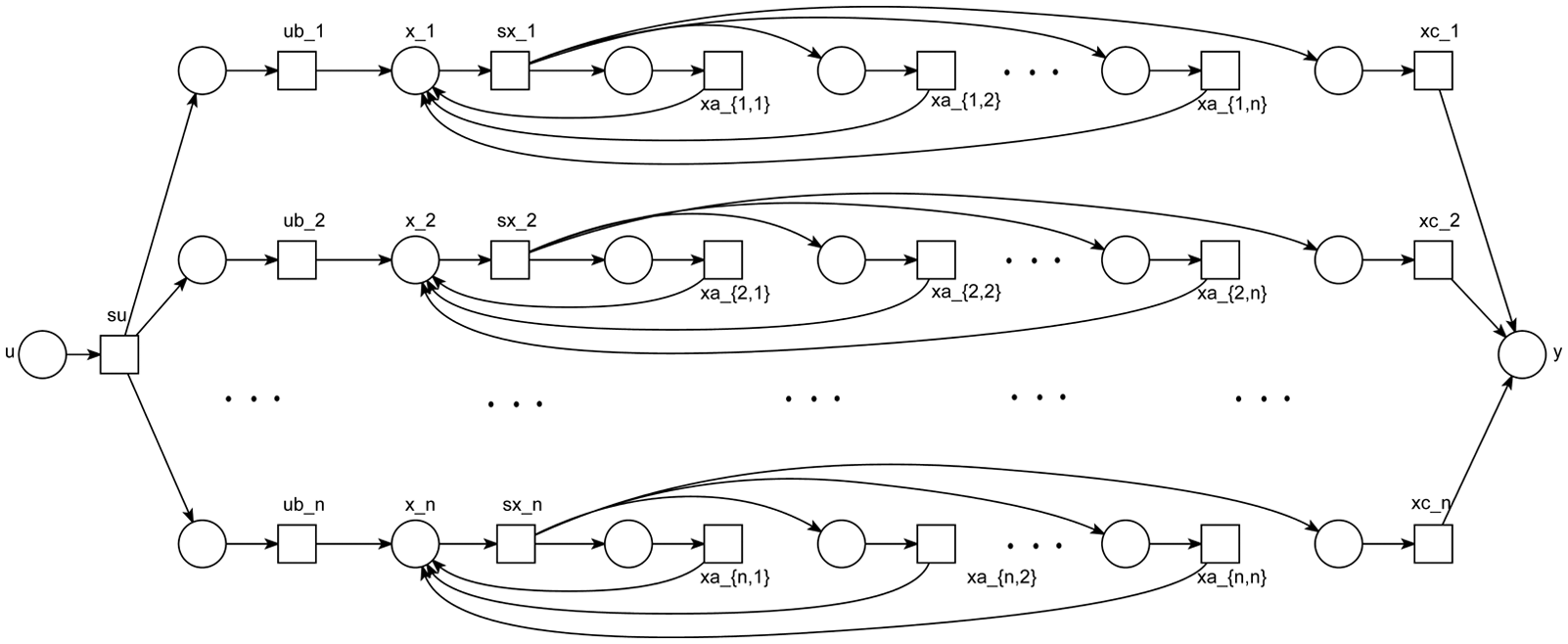
Discrete-time linear control in two tacts.

Note that for any number of states, the values are recalculated in two tacts. In the first tact, all transitions with prefix “sx” fire, splitting their input variables into the required number of copies and saving them in unnamed auxiliary places. In the second tact, all transitions (multiplying by a constant) fire, where a constant with prefix “xa” is attached to their output arcs. Calculating the corresponding sums for multiplications by matrices (or vectors) is done in an implicit way: several transitions put their results into the same output place.

Conclusion

In this publication, the principles of programming in SN language have been further developed with respect to the restrictions on the CF and its composition with data. The conditions for the correctness of SN programs were formulated in the form of additional restrictions on copying parameters of modules and using global variables. Flags were added for correct manipulation by shared data. In the general case, the problem is reduced to the soundness of WFNs with shared resources, which is solved in polynomial time. Programming in SN was illustrated with the example of solving a production control task.

Thus, using the strict composition rules described in this article we obtain a correct (by construction) program written in SNPL. When applying slack rules we have an efficient method for finding deadlocks and enforcing liveness.

Footnotes

Academic Editor: ZhiWu Li

Declaration of conflicting interests

The author(s) declared no potential conflicts of interest with respect to the research, authorship, and/or publication of this article.

Funding

The author(s) disclosed receipt of the following financial support for the research, authorship, and/or publication of this article: The work was supported by a Deutscher Akademischer Austauschdienst (DAAD) fellowship and partially funded by the DFG project SecVolution (JU 2734/2-1) which is part of the priority program SPP 1593 “Design For Future - Managed Software Evolution.”

References

Rumbaugh

Jacobson

Booch

The unified modeling language reference manual. Boston, MA: Addison-Wesley, 1999.

Jürjens

Secure systems development with UML. Berlin: Springer, 2005.

Taubenberger

Jürjens

. Resolving vulnerability identification errors using security requirements on business process models. Inform Manag Comput Secur 2013; 21: 202–223.

Giua

Design of optimal Petri net controllers for disjunctive generalized mutual exclusion constraints. IEEE T Automat Contr 2015; 60: 1774–1785.

Peng

Zhou

. Petri net based PLC stage programming for discrete-event control design. In: Proceedings of the IEEE international conference on systems, man, and cybernetics, 7–10 October 2001, vol. 4, pp.2706–2710. New York: IEEE.

Zaitsev

DA.

Sleptsov nets run fast. IEEE T Syst Man Cy: Syst. Epub ahead of print 1 July 2015. DOI: 10.1109/TSMC.2015.2444414.

Zaitsev

DA.

Toward the minimal universal Petri net. IEEE T Syst Man Cy: Syst 2014; 44: 47–58.

Zaitsev

. Small polynomial time universal Petri nets. arXiv:1309.7288, http://arxiv.org/abs/1309.7288

Zaitsev

DA.

Paradigm of computations on the Petri nets. Automat Rem Contr 2014; 75: 1369–1383.

10.

Berthomieu

Vernadat

Time Petri nets analysis with TINA. In: Proceedings of 3rd international conference on the quantitative evaluation of systems (QEST 2006), Riverside, CA, 11–14 September 2006. New York: IEEE Computer Society.

11.

van der Aalst

VMP

, The application of Petri nets to workflow management. J Circuit Syst Comp 1998; 8: 21–66.

12.

Chen

ZW.

Design of a maximally permissive liveness-enforcing supervisor with a compressed supervisory structure for flexible manufacturing systems. Automatica 2011; 47: 1028–1034.

13.

Barkaoui

Petrucci

Structural analysis of workflow nets with shared resources, 1998, http://citeseerx.ist.psu.edu/viewdoc/download?doi=10.1.1.30.8260&rep=rep1&type=pdf

14.

Bashkin

Lomazova

. Soundness of workflow nets with an unbounded resource is decidable. In: PNSE’13—Petri Nets and Software Engineering, 2013, pp.61–75, http://ceur-ws.org/Vol-989/paper02.pdf

15.

Sidorova

Soundness for resource-constrained workflow nets is decidable. IEEE T Syst Man Cy: Syst 2013; 43: 724–729.

16.

Liu

Sun

Liu

. Complexity of the soundness problem of bounded workflow nets. In: The 33rd international conference on application and theory of Petri nets (Lecture Notes in Computer Science), 25–29 June 2012, vol. 7347, pp.92–107. Berlin: Springer.

17.

Barkaoui

Ayed

Sbai

Workflow soundness verification based on structure theory of Petri nets. Int J Comput Inf Sci 2007; 5: 51–61.

18.

Zhou

ZW.

Short-term scheduling of crude-oil operations: petri net-based control-theoretic approach. IEEE Robot Autom Mag 2015; 22: 64–76.

19.

Chu

. Schedulability analysis of short-term scheduling for crude oil operations in refinery with oil residency time and charging-tank-switch-overlap constraints. IEEE T Autom Sci Eng 2011; 8: 190–204.

20.

Chu

. Hybrid Petri net modeling and schedulability analysis of high fusion point oil transportation under tank grouping strategy for crude oil operations in refinery. IEEE T Syst Man Cy C 2010; 40: 159–175.

21.

Passino

Yurkovich

Fuzzy control. Boston, MA: Addison-Wesley, 1997.

22.

Mengi

Altas

IH.

Fuzzy logic control for a wind/battery renewable energy production system. Turk J Electr Eng Co 2012; 20: 187–206.

23.

Aziz

Wingate

Balas

. Control theory of systems governed by partial differential equations. New York: Academic Press, 2014.

24.

Astrom

Murray Richard

Feedback systems: an introduction for scientists and engineers. Princeton, NJ: Princeton University Press, 2008.

25.

David Ren Alla Hassane . Discrete, continuous, and hybrid Petri nets. Berlin: Springer, 2010.

26.

Sava

Adjallah

Lagaza

. Hybrid Petri nets for modeling and control of multi-source energy conversion systems. In: 2014 international conference on, Control, Decision and Information Technologies (CoDIT), Metz, 3–5 November 2014, pp.516–521. New York: IEEE.

27.

Lewis

AD.

A mathematical approach to classical control. Technical report, Queens University, Kingston, ON, Canada, 2003, http://www.mast.queensu.ca/~andrew/teaching/math332/pdf/332notes.pdf

28.

Haugen

Discrete-time signals and systems. TechTeach, 2005, http://techteach.no/publications/discretetime_signals_systems/discrete.pdf

Programming in the Sleptsov net language for systems control

Abstract

Keywords

Introduction

An overview of SN programming

Properties of the CF of SN programs

Statement 1

Proof

Lemma 1

Proof

Theorem 1

Concurrent data access rules

Closed modules only

Statement 2

Proof

Theorem 2

Proof

Theorem 3

Proof

Basic set of elementary modules for the composition of correct and efficient programs

Correctness of open modules

Theorem 4

Proof

Some notes on deadlock avoidance techniques

Examples of SN programs

Multiplication using a compositional approach

Fast solving production control tasks by SNs

Conclusion

Footnotes

Declaration of conflicting interests

Funding

References