Sage Journals: Discover world-class research

Abstract

This article is concerned with free vibration analysis of open circular cylindrical shells with either the two straight edges or the two curved edges simply supported and the remaining two edges supported by arbitrary classical boundary conditions. An analytical solution of the traveling wave form along the simply supported edges and the standing wave form along the remaining two edges is obtained based on the Flügge thin shell theory. With such a unidirectional traveling wave form solution, the method of reverberation-ray matrix is introduced to derive the equation of natural frequencies of the open circular cylindrical shell with various boundary conditions. Then, the golden section search algorithm is employed to obtain the natural frequencies of the open circular cylindrical shell. The calculation results are compared with those obtained by the finite element method and the method in available literature. Finally, the natural frequencies of the open circular cylindrical shell with various boundary conditions are calculated and the effects of boundary conditions on the natural frequencies are examined. The calculation results can be used as benchmark values for researchers to check their numerical methods and for engineers to design thin structures with shell components.

Keywords

Open circular cylindrical shell method of reverberation-ray matrix free vibration analysis Flügge thin shell theory wave form solution

Introduction

Thin shells are extensively used in naval architecture and ocean engineering, as well as in civil, mechanical, and aeronautical engineering. Open circular cylindrical shells (OCCSs) are often applied as structural components of pressure vessels, roof structures, open space buildings, and marine structures. It is of great significance for engineers to be familiar with vibration behaviors of such shell structures in practical design.

Vibration of OCCSs has been studied by many researchers in the past decades. A comprehensive presentation of the available results for vibration of shell structures was provided by Leissa,¹ in which various theoretical models are presented and the free vibration characteristics of the OCCSs are analyzed. The early researches on OCCSs mainly involve the free vibration analysis with numerical methods such as the Rayleigh–Ritz method,^2–4 the spline finite strip method,⁵ and the finite element method (FEM).^6–10

Ohga et al.¹¹ presented an analytical procedure to estimate natural frequencies and modes of open cylindrical shells with a circumferential thickness taper by the transfer matrix method. The transfer matrix is derived from the nonlinear differential equations for the cylindrical shells by numerical integration. Lim et al.^12,13 proposed a higher order shear deformation theory to investigate the vibratory characteristics of thick cylindrical shallow shells of rectangular planform and then analyzed the effects of various shell geometries and boundary conditions on the vibration responses. Yu et al.¹⁴ obtained exact solutions for OCCSs with simple boundary conditions using the generalized Navier method and accurate solutions for shells with mixed boundary conditions using the method of superposition. Price et al.¹⁵ reviewed the theories of vibration of cylindrical pipes and open shells within the context of thin shell theory. A summary of the thin shell equations of motion and the solutions corresponding to several thin shell theories are presented and applied in a specific example, and the calculation results are compared with those obtained by the FEM. Zhang et al.¹⁶ presented the vibration analysis of cylindrical panels using a wave propagation method. The calculation results are evaluated against those available in the literature. Toorani and Lakis¹⁷ discussed the free vibration of anisotropic laminated composite, as well as isotropic open or closed cylindrical shells submerged in and subjected simultaneously to an internal and external incompressible, inviscid fluid on the basis of a refined shell theory in which transverse shear deformation and rotary inertia effects are taken into account. Gulgazaryan¹⁸ studied natural vibrations localized at the free edge (FE) of a semi-infinite, elastic, orthotropic, circular cylindrical shell of open profile. A variational full-filled method for the free vibration analysis of open circular cylindrical laminated shells supported at discrete points was presented by Singh and Shen,¹⁹ in which a differential equation in matrix form is developed using the first-order shear deformable theory of shells, and rotary inertia is included. Kandasamy and Singh²⁰ presented a numerical study for the free vibration of skewed open circular cylindrical deep shells. Since the formulation is based on the first-order shear deformation theory and includes the rotary inertia, the vibration behaviors of thin to moderately thick shells can be analyzed. Zhang and Xiang,^21,22 respectively, developed an analytical procedure for determining the natural frequencies of OCCSs with stepped thickness variations and with intermediate ring supports based on the Flügge thin shell theory. Gulgazaryan et al.²³ investigated the vibrations of a thin elastic orthotropic circular closed cylindrical shell with free and hinge-mounted ends and of an open cylindrical shell with free and hinge-mounted edges, when the two boundary generatrices are hinge-mounted. Kandasamy and Singh²⁴ presented the free vibration analysis of open skewed circular cylindrical shells supported only on selected segments of the straight edges by means of numerical methods. Wang et al.^25,26 investigated the nonlinear dynamic response of a cantilever rotating circular cylindrical shell subjected to a harmonic excitation about one of the lowest natural frequency and the nonlinear dynamic response in forced oscillations of a third-order nonlinear partial differential system with the method of harmonic balance.

Recently, Ye et al.²⁷ presented a unified Chebyshev–Ritz formulation for the free vibration analysis of open shells with arbitrary boundary conditions and various geometric parameters such as subtended angle and conicity, and the formulation was extended to investigate the vibrations of composite laminated deep open shells with various shell curvatures and arbitrary restraints, including cylindrical, conical, and spherical shells by the subsequent work.²⁸ Su et al.²⁹ presented the free vibration analysis of functionally graded open shells including cylindrical, conical, and spherical shells with arbitrary subtended angle and general boundary conditions.

As far as the authors are concerned, researches on vibration analysis of plate-shell coupled structures are rare, especially for those with analytical methods. For the available literature, the accuracy of the approximate methods is less than that of the analytical methods. While the available analytical methods are sometimes too targeted for shell structures to be consistent with exact solutions of other structural components, such as beams and plates. The method of reverberation-ray matrix (MRRM) is a suitable method for determining natural frequencies and steady-state response of multi-span structures and space frame structures with complex geometry. MRRM was first proposed by Howard and Pao to analyze wave propagation in planar trusses.^30–32 Subsequently, Pao and his associates extended the method to study waves propagating in a multilayered media.^33–38 Many attentions on applications of MRRM were paid to dynamic analysis of frames and beams.^39–51 Meanwhile, MRRM is also employed to analyze unidirectional wave propagation through plates^52–56 and closed shells.^57–59 Recently, the research objects of MRRM turn to be functionally graded or laminated structures.^{50,55,59–62} The unidirectional traveling wave form solution for OCCSs obtained in this article is of good consistency with the solutions for beams and plates presented in literature.^{42,43,47,52,53,58} Therefore, the formulation presented in this article is a fundamental research for vibration analysis of ring-stiffened OCCSs and plate-shell coupled structures.

This article is concerned with an analytical procedure for free vibration analysis of an isotropic OCCS with either the two straight edges or the two curved edges simply supported (SS) and the remaining two edges supported by arbitrary classical boundary conditions. Based on the Flügge thin shell theory, the force and moment resultants and the equations of motion for an OCCS are presented in the beginning. Then, analytical solutions of the traveling wave form along the SS edges and the standing wave form along the remaining two edges are obtained for OCCSs with either two SS straight edges or two SS curved edges. With the solutions expressed in matrix form, the scattering matrix, phase matrix, and permutation matrix as well as the reverberation-ray matrix of the OCCS are derived. Then, the equation of natural frequencies of the OCCS is obtained by MRRM and subsequently solved by the golden section search algorithm.^63,64 The natural frequencies for the OCCS with all four SS edges are obtained by the method presented in this article and the results are compared with those obtained by FEM and the method presented in available literature. Finally, the natural frequencies of the OCCS with various boundary conditions are calculated and the effects of the boundary conditions on the natural frequencies are revealed at the end of this article.

Formulation

Consider an isotropic, OCCS with length L, included angle θ₀, uniform thickness h, middle surface radius R, Young’s modulus E, Poisson’s ratio µ, and mass density ρ, as shown in Figure 1. The axial, circumferential, and radial displacements of the middle surface of the OCCS with reference to the coordinate system are denoted as u(x, θ, t), v(x, θ, t), and w(x, θ, t), respectively. Either the two straight edges or the two curved edges of the shell are assumed to be SS in the following discussions. The problem at hand is to determine the natural frequencies of the OCCS.

Figure 1.

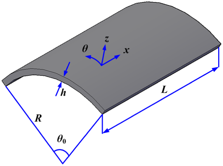
Geometry and coordinate system for an OCCS.

To begin with, the relations of the force and moment resultants with the displacements and the governing equations based on the Flügge thin shell theory are introduced. Subsequently, with the employment of Fourier transform, an analytical solution of the traveling wave form along the SS edges and the standing wave form along the remaining two edges is obtained in the frequency domain. Then, the solutions of the displacements and the force and moment resultants are expressed in matrix form. Finally, the equations of natural frequencies of the OCCS with various classical boundary conditions are obtained by MRRM and solved by the golden section search algorithm. The above-mentioned formulation is presented in detail as follows.

Force and moment resultants

The force and moment resultants in an OCCS, as shown in Figure 2, are expressed in terms of displacement components u, v, and w as follows¹

N_{xx} = \frac{Eh}{1 - μ^{2}} [\frac{\partial u}{\partial x} + μ \frac{1}{R} \frac{\partial v}{\partial θ} - λ R \frac{\partial^{2} w}{\partial x^{2}} + μ \frac{1}{R} w]

(1)

N_{θ θ} = \frac{Eh}{1 - μ^{2}} [μ \frac{\partial u}{\partial x} + \frac{1}{R} \frac{\partial v}{\partial θ} + λ \frac{1}{R} \frac{\partial^{2} w}{\partial θ^{2}} + (1 + λ) \frac{1}{R} w]

(2)

N_{x θ} = \frac{Eh}{2 (1 + μ)} [\frac{1}{R} \frac{\partial u}{\partial θ} + (1 + λ) \frac{\partial v}{\partial x} - λ \frac{\partial^{2} w}{\partial x \partial θ}]

(3)

N_{θ x} = \frac{Eh}{2 (1 + μ)} [(1 + λ) \frac{1}{R} \frac{\partial u}{\partial θ} + \frac{\partial v}{\partial x} + λ \frac{\partial^{2} w}{\partial x \partial θ}]

(4)

M_{xx} = \frac{E h^{3}}{12 (1 - μ^{2})} [\frac{1}{R} \frac{\partial u}{\partial x} + μ \frac{1}{R^{2}} \frac{\partial v}{\partial θ} - \frac{\partial^{2} w}{\partial x^{2}} - μ \frac{1}{R^{2}} \frac{\partial^{2} w}{\partial θ^{2}}]

(5)

M_{θ θ} = \frac{E h^{3}}{12 (1 - μ^{2})} [- μ \frac{\partial^{2} w}{\partial x^{2}} - \frac{1}{R^{2}} \frac{\partial^{2} w}{\partial θ^{2}} - \frac{1}{R^{2}} w]

(6)

M_{x θ} = \frac{E h^{3}}{12 (1 + μ)} (\frac{1}{R} \frac{\partial v}{\partial x} - \frac{1}{R} \frac{\partial^{2} w}{\partial x \partial θ})

(7)

M_{θ x} = \frac{E h^{3}}{12 (1 + μ)} [- \frac{1}{2} \frac{1}{R^{2}} \frac{\partial u}{\partial θ} + \frac{1}{2} \frac{1}{R} \frac{\partial v}{\partial x} - \frac{1}{R} \frac{\partial^{2} w}{\partial x \partial θ}]

(8)

\begin{array}{l} Q_{x z} = \frac{E h^{3}}{12 (1 - μ^{2})} \\ [\frac{1}{R} \frac{\partial^{2} u}{\partial x^{2}} - (1 - μ) \frac{1}{2} \frac{1}{R^{3}} \frac{\partial^{2} u}{\partial θ^{2}} + \frac{1 + μ}{2} \frac{1}{R^{2}} \frac{\partial^{2} v}{\partial x \partial θ} - \frac{\partial^{3} w}{\partial x^{3}} - \frac{1}{R^{2}} \frac{\partial^{3} w}{\partial x \partial θ^{2}}] \end{array}

(9)

\begin{array}{l} Q_{θ z} = \frac{E h^{3}}{12 (1 - μ^{2})} \\ [(1 - μ) \frac{1}{R} \frac{\partial^{2} v}{\partial x^{2}} - \frac{1}{R} \frac{\partial^{3} w}{\partial x^{2} \partial θ} - \frac{1}{R^{3}} \frac{\partial^{3} w}{\partial θ^{3}} - \frac{1}{R^{3}} \frac{\partial w}{\partial θ}] \end{array}

(10)

\begin{array}{l} F_{x θ} = N_{x θ} + \frac{1}{R} M_{x θ} = \frac{E h}{2 (1 + μ)} \\ [\frac{1}{R} \frac{\partial u}{\partial θ} + (1 + 3 λ) \frac{\partial v}{\partial x} - 3 λ \frac{\partial^{2} w}{\partial x \partial θ}] \end{array}

(11)

F_{θ x} = N_{θ x} = \frac{Eh}{2 (1 + μ)} [(1 + λ) \frac{1}{R} \frac{\partial u}{\partial θ} + \frac{\partial v}{\partial x} + λ \frac{\partial^{2} w}{\partial x \partial θ}]

(12)

\begin{array}{l} V_{x z} = Q_{x z} + \frac{1}{R} \frac{\partial M_{x θ}}{\partial θ} = \frac{E h^{3}}{12 (1 - μ^{2})} \\ [\begin{array}{l} \frac{1}{R} \frac{\partial^{2} u}{\partial x^{2}} - (1 - μ) \frac{1}{2} \frac{1}{R^{3}} \frac{\partial^{2} u}{\partial θ^{2}} + \frac{3 - μ}{2} \frac{1}{R^{2}} \frac{\partial^{2} v}{\partial x \partial θ} \\ - \frac{\partial^{3} w}{\partial x^{3}} - (2 - μ) \frac{1}{R^{2}} \frac{\partial^{3} w}{\partial x \partial θ^{2}} \end{array}] \end{array}

(13)

\begin{array}{l} V_{θ z} = Q_{θ z} + \frac{\partial M_{θ x}}{\partial x} = \frac{E h^{3}}{12 (1 - μ^{2})} \\ [\begin{array}{l} - \frac{1 - μ}{2} \frac{1}{R^{2}} \frac{\partial^{2} u}{\partial x \partial θ} + \frac{3 (1 - μ)}{2} \frac{1}{R} \frac{\partial^{2} v}{\partial x^{2}} \\ - (2 - μ) \frac{1}{R} \frac{\partial^{3} w}{\partial x^{2} \partial θ} - \frac{1}{R^{3}} \frac{\partial^{3} w}{\partial θ^{3}} - \frac{1}{R^{3}} \frac{\partial w}{\partial θ} \end{array}] \end{array}

(14)

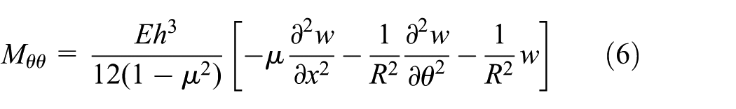
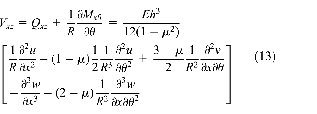
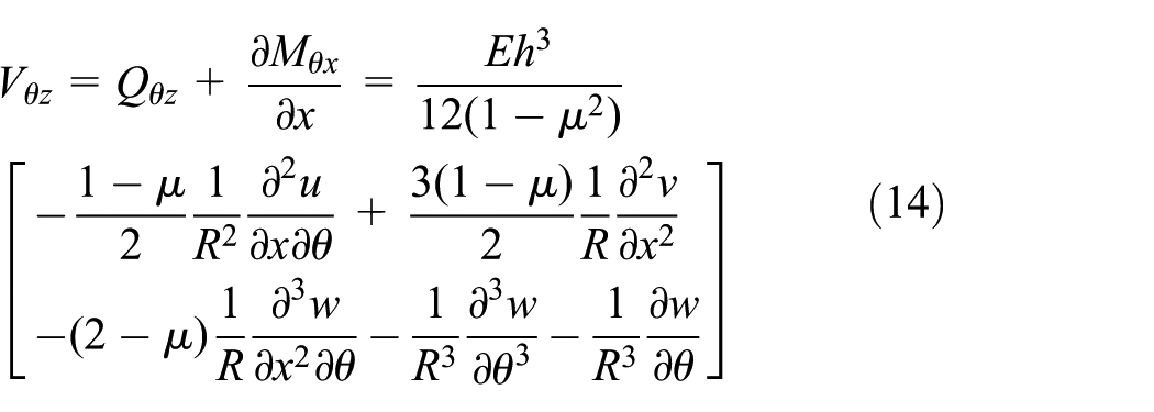
where u, v, and w denote the displacement components in the axial (x), circumferential (θ), and radial (z) directions, respectively. C = Eh/(1 − µ²) and D = Eh³/12(1 − µ²) represent the middle surface stiffness and the bending stiffness of the shell, respectively. N_xx and N_θθ denote the in-plane normal forces, N_xθ and N_θx the in-plane shear forces, M_xx and M_θθ the bending moment, M_xθ and M_θx the torsional moment, and Q_xz and Q_θz the out-of-plane shear forces acting on the cross sections perpendicular to the axial and circumferential directions, respectively. Besides, F_xθ and F_θx indicate the in-plane shear force resultants and V_xz and V_θz the out-of-plane shear force resultants acting on the cross sections perpendicular to the axial and circumferential directions, respectively.

Figure 2.

Force and moment resultants in a shell (positive directions are indicated).

Governing differential equations

Based on the Flügge thin shell theory, the governing differential equations for free vibration of an OCCS are written as^1,65

\begin{matrix} R^{2} \frac{\partial^{2} u}{\partial x^{2}} & + (1 + λ) \frac{1 - μ}{2} \frac{\partial^{2} u}{\partial θ^{2}} + \frac{1 + μ}{2} R \frac{\partial^{2} v}{\partial x \partial θ} \\ - λ R^{3} \frac{\partial^{3} w}{\partial x^{3}} + λ \frac{1 - μ}{2} R \frac{\partial^{3} w}{\partial x \partial θ^{2}} \\ + μ R \frac{\partial w}{\partial x} - R^{2} \frac{ρ (1 - μ^{2})}{E} \frac{\partial^{2} u}{\partial t^{2}} = 0 \end{matrix}

(15)

\begin{array}{l} \frac{1 + μ}{2} R \frac{\partial^{2} u}{\partial x \partial θ} + (1 + 3 λ) \frac{1 - μ}{2} \\ R^{2} \frac{\partial^{2} v}{\partial x^{2}} + \frac{\partial^{2} v}{\partial θ^{2}} - λ \frac{3 - μ}{2} R^{2} \frac{\partial^{3} w}{\partial x^{2} \partial θ} \\ + \frac{\partial w}{\partial θ} - R^{2} \frac{ρ (1 - μ^{2})}{E} \frac{\partial^{2} v}{\partial t^{2}} = 0 \end{array}

(16)

\begin{matrix} - λ R^{3} \frac{\partial^{3} u}{\partial x^{3}} + λ \frac{1 - μ}{2} R \frac{\partial^{3} u}{\partial x \partial θ^{2}} + μ R \frac{\partial u}{\partial x} \\ - \frac{3 - μ}{2} λ R^{2} \frac{\partial^{3} v}{\partial x^{2} \partial θ} + \frac{\partial v}{\partial θ} \\ + λ R^{4} \frac{\partial^{4} w}{\partial x^{4}} + 2 λ R^{2} \frac{\partial^{4} w}{\partial x^{2} \partial θ^{2}} + λ \frac{\partial^{4} w}{\partial θ^{4}} + 2 λ \frac{\partial^{2} w}{\partial θ^{2}} \\ + (1 + λ) w + R^{2} \frac{ρ (1 - μ^{2})}{E} \frac{\partial^{2} w}{\partial t^{2}} = 0 \end{matrix}

(17)

where λ = h²/12R² is a dimensionless parameter, which is related to the ratio of the shell thickness to shell radius.

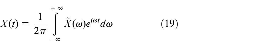
The Fourier transform of an arbitrary physical quantity X(t) is defined as

\tilde{X} (ω) = \int_{- \infty}^{+ \infty} X (t) e^{- i ω t} dt

(18)

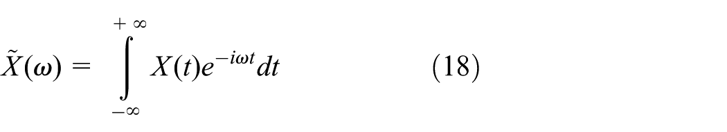
where ω is the circular frequency, and a tilde over a symbol represents the corresponding quantity expressed in the frequency domain. The inverse Fourier transform is given by

X (t) = \frac{1}{2 π} \int_{- \infty}^{+ \infty} \tilde{X} (ω) e^{i ω t} d ω

(19)

Taking the Fourier transforms of equations (15)–(17), the governing differential equations can be expressed in the frequency domain as

\begin{matrix} R^{2} \frac{\partial^{2}}{\partial x^{2}} \tilde{u} + (1 + λ) \frac{1 - μ}{2} \frac{\partial^{2}}{\partial θ^{2}} \tilde{u} + R^{2} k_{L}^{2} \tilde{u} + \frac{1 + μ}{2} R \frac{\partial^{2}}{\partial x \partial θ} \tilde{v} \\ - λ R^{3} \frac{\partial^{3}}{\partial x^{3}} \tilde{w} + λ \frac{1 - μ}{2} R \frac{\partial^{3}}{\partial x \partial θ^{2}} \tilde{w} + μ R \frac{\partial}{\partial x} \tilde{w} = 0 \end{matrix}

(20)

\begin{array}{l} \frac{1 + μ}{2} R \frac{\partial^{2}}{\partial x \partial θ} \tilde{u} + (1 + 3 λ) \frac{1 - μ}{2} R^{2} \frac{\partial^{2}}{\partial x^{2}} \tilde{v} + \\ \frac{\partial^{2}}{\partial θ^{2}} \tilde{v} + R^{2} k_{L}^{2} \tilde{v} - λ \frac{3 - μ}{2} R^{2} \frac{\partial^{3}}{\partial x^{2} \partial θ} \tilde{w} + \frac{\partial}{\partial θ} \tilde{w} = 0 \end{array}

(21)

\begin{matrix} - λ R^{3} \frac{\partial^{3}}{\partial x^{3}} \tilde{u} + λ \frac{1 - μ}{2} R \frac{\partial^{3}}{\partial x \partial θ^{2}} \tilde{u} + μ R \frac{\partial}{\partial x} \tilde{u} \\ - \frac{3 - μ}{2} λ R^{2} \frac{\partial^{3}}{\partial x^{2} \partial θ} \tilde{v} + \frac{\partial}{\partial θ} \tilde{v} \\ + λ R^{4} \frac{\partial^{4}}{\partial x^{4}} \tilde{w} + 2 λ R^{2} \frac{\partial^{4}}{\partial x^{2} \partial θ^{2}} \tilde{w} + λ \frac{\partial^{4}}{\partial θ^{4}} \tilde{w} \\ + 2 λ \frac{\partial^{2}}{\partial θ^{2}} \tilde{w} + (1 + λ) \tilde{w} - R^{2} k_{L}^{2} \tilde{w} = 0 \end{matrix}

(22)

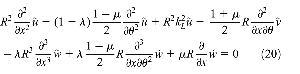
where k_L = ω[(1 − µ²)ρ/E]^1/2 represents the in-plane longitudinal wave number.

Equations (20)–(22) can be represented in linear differential operator form as

L_{4} \tilde{u} + L_{3} \tilde{v} + L_{5} R \frac{\partial}{\partial x} \tilde{w} = 0

(23)

L_{3} \tilde{u} + L_{6} \tilde{v} + L_{7} \frac{\partial}{\partial θ} \tilde{w} = 0

(24)

L_{5} R \frac{\partial}{\partial x} \tilde{u} + L_{7} \frac{\partial}{\partial θ} \tilde{v} + L_{8} \tilde{w} = 0

(25)

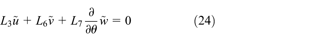
Substituting equation (23) into equation (24) and eliminating the circumferential displacement $\tilde{v}$ yields

(L_{4} L_{6} - L_{3} L_{3}) \tilde{u} = (L_{2} L_{7} - L_{5} L_{6}) R \frac{\partial}{\partial x} \tilde{w}

(26)

Substituting equation (23) into equation (24) and eliminating the axial displacement $\tilde{u}$ yields

(L_{4} L_{6} - L_{3} L_{3}) \tilde{v} = (L_{1} L_{5} - L_{4} L_{7}) \frac{\partial}{\partial θ} \tilde{w}

(27)

Similarly, substituting equation (23) into equation (25) and eliminating the circumferential displacement $\tilde{v}$ yields

- (L_{1} L_{5} - L_{4} L_{7}) \frac{\partial}{\partial θ} \tilde{u} = (\frac{1 + μ}{2} L_{8} - L_{5} L_{7}) R \frac{\partial^{2}}{\partial x \partial θ} \tilde{w}

(28)

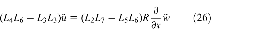
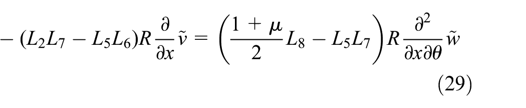
Substituting equation (24) into equation (25) and eliminating the axial displacement $\tilde{u}$ yields

- (L_{2} L_{7} - L_{5} L_{6}) R \frac{\partial}{\partial x} \tilde{v} = (\frac{1 + μ}{2} L_{8} - L_{5} L_{7}) R \frac{\partial^{2}}{\partial x \partial θ} \tilde{w}

(29)

All the above-mentioned linear differential operators L_j (j = 1–8) are presented in detail in section “Linear differential operators L_i” in Appendix 1.

Subsequently, substituting equation (26) into equation (28) and eliminating the radial displacement $\tilde{w}$ yields

[(L_{4} L_{6} - L_{3} L_{3}) (\frac{1 + μ}{2} L_{8} - L_{5} L_{7}) + (L_{1} L_{5} - L_{4} L_{7}) (L_{2} L_{7} - L_{5} L_{6})] \frac{\partial}{\partial θ} \tilde{u} = 0

(30)

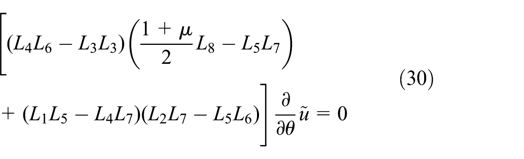
In a similar manner, substituting equation (27) into equation (29) and eliminating the radial displacement $\tilde{w}$ results in

[(L_{4} L_{6} - L_{3} L_{3}) (\frac{1 + μ}{2} L_{8} - L_{5} L_{7}) + (L_{1} L_{5} - L_{4} L_{7}) (L_{2} L_{7} - L_{5} L_{6})] R \frac{\partial}{\partial x} \tilde{v} = 0

(31)

However, with the radial displacement $\tilde{w}$ reserved, substitution of equation (26) into equation (28) or equation (27) into equation (29) yields

[(L_{4} L_{6} - L_{3} L_{3}) (\frac{1 + μ}{2} L_{8} - L_{5} L_{7}) + (L_{1} L_{5} - L_{4} L_{7}) (L_{2} L_{7} - L_{5} L_{6})] R \frac{\partial^{2}}{\partial x \partial θ} \tilde{w} = 0

(32)

It can be observed from equations (30)–(32) that the differences among the linear differential operators operating on the axial, circumferential, and radial displacement components lie in the parts outside the braces, which represent zero wave number solutions, or in other words, the rigid-body motions. As is the case in free vibration analysis, the zero wave number solutions will be neglected throughout this article.

Solutions for the OCCS with the curved edges supported by SSs

As the two curved edges of the OCCS are assumed to be SS, the boundary conditions at x = 0 and x = L are given by¹

v = 0, w = 0, N_{xx} = 0, M_{xx} = 0, x = 0, L

(33)

According to the boundary conditions defined by equation (33), the axial, circumferential, and radial displacements of the OCCS can be expressed as

\tilde{u} (x, θ) = \sum_{m = 1}^{\infty} U (θ) \cos (k_{x} x)

(34)

\tilde{v} (x, θ) = \sum_{m = 1}^{\infty} V (θ) \sin (k_{x} x)

(35)

\tilde{w} (x, θ) = \sum_{m = 1}^{\infty} W (θ) \sin (k_{x} x)

(36)

where k_x = mπ/L denotes the wave number in the axial direction, m is the axial mode number, and L represents the length of the OCCS.

Assuming that the axial, circumferential, and radial displacements can be expressed as exponential functions of the circumferential variable θ, a common circumferential wave number equation for the axial, circumferential, and radial displacements of the OCCS is obtained

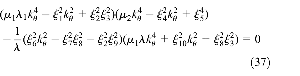
\begin{array}{l} (μ_{1} λ_{1} k_{θ}^{4} - ξ_{1}^{2} k_{θ}^{2} + ξ_{2}^{2} ξ_{3}^{2}) (μ_{2} k_{θ}^{4} - ξ_{4}^{2} k_{θ}^{2} + ξ_{5}^{4}) \\ - \frac{1}{λ} (ξ_{6}^{2} k_{θ}^{2} - ξ_{7}^{2} ξ_{8}^{2} - ξ_{2}^{2} ξ_{9}^{2}) (μ_{1} λ k_{θ}^{4} + ξ_{10}^{2} k_{θ}^{2} + ξ_{8}^{2} ξ_{3}^{2}) = 0 \end{array}

(37)

where µ_j (j = 1, 2), λ₁ and ξ_j (j = 1–10) are the non-dimensional parameters presented in detail in sections “Dimensionless parameters µ_j and λ_j” and “Dimensionless parameters ξ_j” in Appendix 1.

By solving equation (37), eight circumferential wave numbers are obtained

k_{θ} = \pm k_{θ 1}, \pm k_{θ 2}, \pm k_{θ 3}, \pm k_{θ 4}

(38)

Therefore, the solutions of the equations of motion of the OCCS with two SS curved edges are expressed in the frequency domain as

\tilde{u} (x, θ) = \sum_{m = 1}^{\infty} \sum_{j = 1}^{4} α_{j} (a_{j} e^{i k_{θ j} θ} + d_{j} e^{- i k_{θ j} θ}) \cos (k_{x} x)

(39)

\tilde{v} (x, θ) = \sum_{m = 1}^{\infty} \sum_{j = 1}^{4} β_{j} (a_{j} e^{i k_{θ j} θ} - d_{j} e^{- i k_{θ j} θ}) \sin (k_{x} x)

(40)

\tilde{w} (x, θ) = \sum_{m = 1}^{\infty} \sum_{j = 1}^{4} (a_{j} e^{i k_{θ j} θ} + d_{j} e^{- i k_{θ j} θ}) \sin (k_{x} x)

(41)

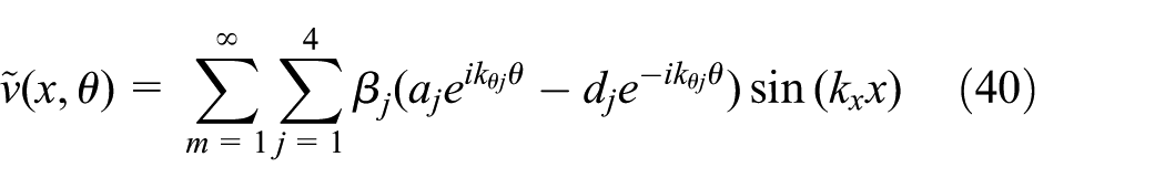
where α_j and β_j (j = 1–4) are the ratios of the amplitude coefficients of the axial and circumferential displacements to the amplitude coefficient of the radial displacement, respectively. The expressions of α_j and β_j are presented as follows

α_{j} = - R k_{x} (μ_{2} λ k_{θ j}^{4} + ξ_{10}^{2} k_{θ j}^{2} + ξ_{3}^{2} ξ_{8}^{2}) / (μ_{2} λ_{1} k_{θ j}^{4} - ξ_{1}^{2} k_{θ j}^{2} + ξ_{2}^{2} ξ_{3}^{2})

(42)

β_{j} = i k_{θ j} (ξ_{6}^{2} k_{θ j}^{2} - ξ_{7}^{2} ξ_{8}^{2} - ξ_{2}^{2} ξ_{9}^{2}) / (μ_{2} λ_{1} k_{θ j}^{4} - ξ_{1}^{2} k_{θ j}^{2} + ξ_{2}^{2} ξ_{3}^{2})

(43)

The rotation of the normal to the middle surface of the OCCS about the axial direction is defined as

ϕ_{θ} = \frac{v}{R} - \frac{\partial w}{R \partial θ}

(44)

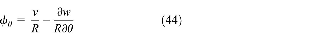
According to equations (40) and (41), the above-mentioned rotation can be expressed in frequency domain as

{\tilde{ϕ}}_{θ} = \sum_{m = 1}^{\infty} \sum_{j = 1}^{4} \frac{1}{R} (β_{j} - i k_{θ j}) (a_{j} e^{i k_{θ j} θ} - d_{j} e^{- i k_{θ j} θ}) \sin (k_{x} x)

(45)

Besides, substitution of equations (39)–(41) into the Fourier transforms of equations (2), (6), (12), and (14) yields the frequency domain expressions of the force and moment resultants of the OCCS

\begin{matrix} {\tilde{N}}_{θ θ} = \frac{C}{R} \sum_{m = 1}^{\infty} \sum_{j = 1}^{4} \\ {[λ_{1} - λ k_{θ j}^{2} - μ R k_{x} α_{j} + i k_{θ j} β_{j}] (a_{j} e^{i k_{θ j} θ} + d_{j} e^{- i k_{θ j} θ})} \sin (k_{x} x) \end{matrix}

(46)

\begin{matrix} {\tilde{M}}_{θ θ} = - \frac{D}{R^{2}} \sum_{m = 1}^{\infty} \sum_{j = 1}^{4} \\ [(1 - k_{θ j}^{2} - μ R^{2} k_{x}^{2}) (a_{j} e^{i k_{θ j} θ} + d_{j} e^{- i k_{θ j} θ})] \sin (k_{x} x) \end{matrix}

(47)

{\tilde{F}}_{θ x} = \frac{1 - μ}{2 R} C \sum_{m = 1}^{\infty} \sum_{i = 1}^{4} (λ R k_{x} i k_{θ j} + λ_{1} i k_{θ j} α_{j} + R k_{x} β_{j}) (a_{j} e^{i k_{θ j} θ} - d_{j} e^{- i k_{θ j} θ}) \cos (k_{x} x)

(48)

{\tilde{V}}_{θ z} = \frac{D}{R^{3}} \sum_{m = 1}^{\infty} \sum_{j = 1}^{4} [\begin{array}{l} (2 - μ) R^{2} k_{x}^{2} i k_{θ j} + i k_{θ j}^{3} - i k_{θ j} \\ + μ_{2} R k_{x} i k_{θ j} α_{j} - 3 μ_{2} R^{2} k_{x}^{2} β_{j} \end{array}] (a_{j} e^{i k_{θ j} θ} - d_{j} e^{- i k_{θ j} θ}) \sin (k_{x} x)

(49)

Solutions for the OCCS with SS straight edges

Since the derivation for solutions of the OCCS with SS straight edges is independent of the derivation for the OCCS with SS curved edges and the two derivation procedures are quite similar to each other, the symbols used in this section will be very similar and frequently the same to those used in the preceding section.

As the two straight edges of the OCCS are assumed to be SS, the boundary conditions at θ = 0 and θ = θ₀ are given by¹

u = 0, w = 0, N_{θ θ} = 0, M_{θ θ} = 0, θ = 0, θ_{0}

(50)

According to the boundary conditions defined by equation (50), the axial, circumferential, and radial displacements of the OCCS are written as

\tilde{u} (x, θ) = \sum_{n = 1}^{\infty} U (x) \sin (k_{θ} θ)

(51)

\tilde{v} (x, θ) = \sum_{n = 1}^{\infty} V (x) \cos (k_{θ} θ)

(52)

\tilde{w} (x, θ) = \sum_{n = 1}^{\infty} W (x) \sin (k_{θ} θ)

(53)

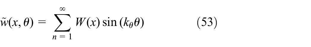
where k_θ = nπ/θ₀ denotes the circumferential wave number, n is the mode number, and θ₀ represents the included angle of the OCCS.

Assuming that the axial, circumferential, and radial displacements are expressed as exponential functions of the axial variable x, a common axial wave number equation of the axial, circumferential, and radial displacements of the OCCS can be obtained as

\begin{array}{l} (λ_{2} μ_{2} k_{x}^{4} - ζ_{1}^{2} k_{x}^{2} + ζ_{2}^{2} ζ_{3}^{2}) (λ_{3} k_{x}^{4} - ζ_{4}^{2} k_{x}^{2} + ζ_{5}^{4}) \\ + \frac{1}{λ} (2 λ μ_{2} k_{x}^{4} - ζ_{6}^{2} k_{x}^{2} - ζ_{2}^{2} ζ_{7}^{2}) (λ λ_{2} μ_{2} k_{x}^{4} - ζ_{8}^{2} k_{x}^{2} + ζ_{9}^{4}) = 0 \end{array}

(54)

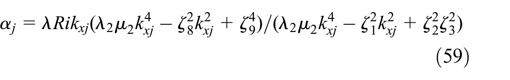
where µ₂ and λ_j (j = 2, 3) are the non-dimensional parameters presented in detail in section “Dimensionless parameters µ_j and λ_j” in Appendix 1. While ζ_j (j = 1–9) are the dimensional parameters of the same dimension as the axial wave number, and they are presented in detail in section “Dimensional parameters ζ_j” in Appendix 1.

By solving equation (54), eight axial wave numbers are obtained

k_{x} = \pm k_{x 1}, \pm k_{x 2}, \pm k_{x 3}, \pm k_{x 4}

(55)

Thus, with respect to the boundary conditions defined by equation (50), the solutions of equations (30)–(32) are written as

\tilde{u} (x, θ) = \sum_{n = 1}^{\infty} \sum_{j = 1}^{4} α_{j} (a_{j} e^{i k_{xj} x} - d_{j} e^{- i k_{xj} x}) \sin (k_{θ} θ)

(56)

\tilde{v} (x, θ) = \sum_{n = 1}^{\infty} \sum_{j = 1}^{4} β_{j} (a_{j} e^{i k_{xj} x} + d_{j} e^{- i k_{xj} x}) \cos (k_{θ} θ)

(57)

\tilde{w} (x, θ) = \sum_{n = 1}^{\infty} \sum_{j = 1}^{4} (a_{j} e^{i k_{xj} x} + d_{j} e^{- i k_{xj} x}) \sin (k_{θ} θ)

(58)

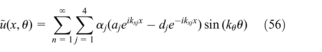
where α_j and β_j (j = 1–4) are the ratios of amplitude coefficients of the axial and circumferential displacements to the amplitude coefficient of the radial displacement. The expressions of α_j and β_j are presented as follows

α_{j} = λ Ri k_{xj} (λ_{2} μ_{2} k_{xj}^{4} - ζ_{8}^{2} k_{xj}^{2} + ζ_{9}^{4}) / (λ_{2} μ_{2} k_{xj}^{4} - ζ_{1}^{2} k_{xj}^{2} + ζ_{2}^{2} ζ_{3}^{2})

(59)

β_{j} = λ k_{θ} (2 μ_{2} k_{xj}^{4} - ζ_{6}^{2} k_{xj}^{2} - ζ_{2}^{2} ζ_{7}^{2}) / (λ_{2} μ_{2} k_{xj}^{4} - ζ_{1}^{2} k_{xj}^{2} + ζ_{2}^{2} ζ_{3}^{2})

(60)

The rotation of the normal to the middle surface about the circumferential direction is defined as

ϕ_{x} = - \frac{\partial w}{\partial x}

(61)

According to equation (61), the above-mentioned rotation is expressed in frequency domain as

{\tilde{ϕ}}_{x} = \sum_{n = 1}^{\infty} \sum_{j = 1}^{4} - i k_{xj} (a_{j} e^{i k_{xj} x} - d_{j} e^{- i k_{xj} x}) \sin (k_{θ} θ)

(62)

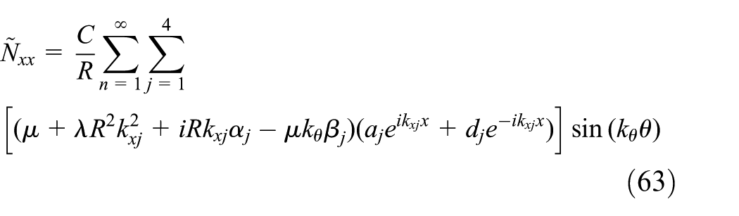
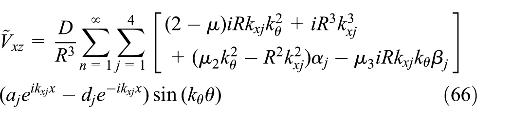
Substituting equations (56)–(58) into the Fourier transforms of equations (1), (5), (11), and (13) yields the frequency domain expressions of the force and moment resultants of the OCCS

{\tilde{N}}_{x x} = \frac{C}{R} \sum_{n = 1}^{\infty} \sum_{j = 1}^{4} [(μ + λ R^{2} k_{x j}^{2} + i R k_{x j} α_{j} - μ k_{θ} β_{j}) (a_{j} e^{i k_{x j} x} + d_{j} e^{- i k_{x j} x})] \sin (k_{θ} θ)

(63)

\begin{matrix} {\tilde{M}}_{xx} = \frac{D}{R^{2}} \sum_{n = 1}^{\infty} \sum_{j = 1}^{4} \\ [(μ k_{θ}^{2} + R^{2} k_{xj}^{2} + iR k_{xj} α_{j} - μ k_{θ} β_{j}) (a_{j} e^{i k_{xj} x} + d_{j} e^{- i k_{xj} x})] \sin (k_{θ} θ) \end{matrix}

(64)

\begin{matrix} {\tilde{F}}_{x θ} = μ_{2} \frac{C}{R} \sum_{n = 1}^{\infty} \sum_{j = 1}^{4} \\ {[- 3 λ iR k_{xj} k_{θ} + k_{θ} α_{j} + λ_{2} iR k_{xj} β_{j}] (a_{j} e^{i k_{xj} x} - d_{j} e^{- i k_{xj} x})} \cos (k_{θ} θ) \end{matrix}

(65)

\begin{array}{l} {\tilde{V}}_{x z} = \frac{D}{R^{3}} \\ \sum_{n = 1}^{\infty} \sum_{j = 1}^{4} [\begin{array}{l} (2 - μ) i R k_{x j} k_{θ}^{2} + i R^{3} k_{x j}^{3} \\ + (μ_{2} k_{θ}^{2} - R^{2} k_{x j}^{2}) α_{j} - μ_{3} i R k_{x j} k_{θ} β_{j} \end{array}] (a_{j} e^{i k_{x j} x} - d_{j} e^{- i k_{x j} x}) \sin (k_{θ} θ) \end{array}

(66)

Solutions expressed in matrix form

SS curved edges

For an arbitrary axial mode number m, equations (39)–(41) and (45) can be expressed in matrix form as

W_{d} = H_{m} (x) W_{d}^{*}

(67)

where W _d denotes the displacement vector of the OCCS, H _m(x) indicates the axial mode matrix, and W _d^* represents the displacement wave vector of the circumferential variable. They are presented in detail as follows

W_{d} = {\begin{matrix} \tilde{u} & \tilde{v} & \tilde{w} & {\tilde{ϕ}}_{θ} \end{matrix}}^{T}

(68)

H_{m} (x) = diag {\begin{matrix} \cos (k_{x} x) & \sin (k_{x} x) & \sin (k_{x} x) & \sin (k_{x} x) \end{matrix}}

(69)

W_{d}^{*} = A_{d} P_{h} (θ) a + D_{d} P_{h} (- θ) d

(70)

in which P _h(θ) denotes the phase matrix, A _d and D _d are the coefficient matrices of fourth order, and a and d are the amplitude vectors of the arriving wave and the departing wave corresponding to the displacements of the OCCS, respectively. They are presented in detail as follows

P_{h} (θ) = diag {\begin{matrix} e^{i k_{θ 1} θ} & e^{i k_{θ 2} θ} & e^{i k_{θ 3} θ} & e^{i k_{θ 4} θ} \end{matrix}}

(71)

a = {\begin{matrix} a_{1} & a_{2} & a_{3} & a_{4} \end{matrix}}^{T}

(72)

d = {\begin{matrix} d_{1} & d_{2} & d_{3} & d_{4} \end{matrix}}^{T}

(73)

\begin{matrix} A_{d} (1, j) = D_{d} (1, j) = α_{j} \\ A_{d} (2, j) = - D_{d} (2, j) = β_{j} \\ A_{d} (3, j) = D_{d} (3, j) = 1 \\ A_{d} (4, j) = - D_{d} (4, j) = (β_{j} - i k_{θ j}) / R \end{matrix}

(74)

where j = 1, 2, 3, 4.

Meanwhile, equations (46)–(49) can be expressed in matrix form as

W_{f} = H_{m} (x) W_{f}^{*}

(75)

where H _m(x) is defined by equation (69), W _f denotes the force vector of the shell, and W _f^* represents the force and moment resultant wave vector of the circumferential variable. They are presented in detail as follows

W_{f} = {\begin{matrix} {\tilde{F}}_{θ x} & {\tilde{N}}_{θ θ} & {\tilde{V}}_{θ z} & {\tilde{M}}_{θ θ} \end{matrix}}^{T}

(76)

W_{f}^{*} = A_{f} P_{h} (θ) a + D_{f} P_{h} (- θ) d

(77)

in which the physical significances and expressions of P _h(θ), a , and d are the same as those presented in equation (70). A _f and D _f are the coefficient matrices corresponding to the arriving wave and the departing wave of the force and moment resultants of the OCCS, respectively. The elements of the coefficient matrices A _f and D _f are listed as follows

\begin{matrix} A_{f} (1, j) & = - D_{f} (1, j) \\ = [λ R k_{x} i k_{θ j} + λ_{1} i k_{θ j} α_{j} + R k_{x} β_{j}] μ_{2} C / R \\ A_{f} (2, j) & = D_{f} (2, j) \\ = (λ_{1} - λ k_{θ j}^{2} - μ R k_{x} α_{j} + i k_{θ j} β_{j}) C / R \\ A_{f} (3, j) & = - D_{f} (3, j) \\ = [(2 - μ) R^{2} k_{x}^{2} i k_{θ j} + μ_{2} R k_{x} i k_{θ j} α_{j} - 3 μ_{2} R^{2} k_{x}^{2} β_{j} + {ik}_{θ j}^{3} - i k_{θ j}] D / R^{3} \\ A_{f} (4, j) & = D_{f} (4, j) = - (1 - k_{θ j}^{2} - μ R^{2} k_{x}^{2}) D / R^{2} \end{matrix}

(78)

where j = 1, 2, 3, 4.

SS straight edges

For an arbitrary circumferential mode number n, equations (56)–(58) and (62) can be rewritten in the same matrix form as equation (67) only if the element ${\tilde{ϕ}}_{θ}$ in W _d is replaced by ${\tilde{ϕ}}_{x}$ and the axial mode matrix H _m(x) and the phase matrix P _h(θ) are replaced by the circumferential mode matrix H _n(θ) and the phase matrix P _h(x), which are defined as follows

H_{n} (θ) = diag {\begin{matrix} \sin (k_{θ} θ) & \cos (k_{θ} θ) & \sin (k_{θ} θ) & \sin (k_{θ} θ) \end{matrix}}

(79)

P_{h} (x) = diag {\begin{matrix} e^{i k_{x 1} x} & e^{i k_{x 2} x} & e^{i k_{x 3} x} & e^{i k_{x 4} x} \end{matrix}}

(80)

Besides, the elements of the coefficient matrices A _d and D _d are replaced by

\begin{matrix} A_{d} (1, j) = - D_{d} (1, j) = α_{j} \\ A_{d} (2, j) = D_{d} (2, j) = β_{j} \\ A_{d} (3, j) = D_{d} (3, j) = 1 \\ A_{d} (4, j) = - D_{d} (4, j) = - i k_{xj} \end{matrix}

(81)

where j = 1, 2, 3, 4.

In a same manner, equations (63)–(66) can be written in the same matrix form as equation (75) only if the axial mode matrix H _m(x) and the phase matrix P _h(θ) are replaced by the circumferential mode matrix H _n(θ) and the phase matrix P _h(x), and the force vector W _f turns to be

W_{f} = {\begin{matrix} {\tilde{F}}_{x θ} & {\tilde{N}}_{xx} & {\tilde{V}}_{xz} & {\tilde{M}}_{xx} \end{matrix}}^{T}

(82)

Besides, the elements of the coefficient matrices A _f and D _f are replaced by

\begin{matrix} A_{f} (1, j) & = D_{f} (1, j) \\ = (μ + λ R^{2} k_{xj}^{2} + iR k_{xj} α_{j} - μ k_{θ} β_{j}) C / R \\ A_{f} (2, j) & = - D_{f} (2, j) \\ = [- 3 λ iR k_{xj} k_{θ} + k_{θ} α_{j} + λ_{2} iR k_{xj} β_{j}] μ_{2} C / R \\ A_{f} (3, j) & = - D_{f} (3, j) \\ = [(2 - μ) iR k_{xj} k_{θ}^{2} + i R^{3} k_{xj}^{3} + (μ_{2} k_{θ}^{2} - R^{2} k_{xj}^{2}) α_{j} - μ_{3} iR k_{xj} k_{θ} β_{j}] D / R^{3} \\ A_{f} (4, j) & = D_{f} (4, j) \\ = (μ k_{θ}^{2} + R^{2} k_{xj}^{2} + iR k_{xj} α_{j} - μ k_{θ} β_{j}) D / R^{2} \end{matrix}

(83)

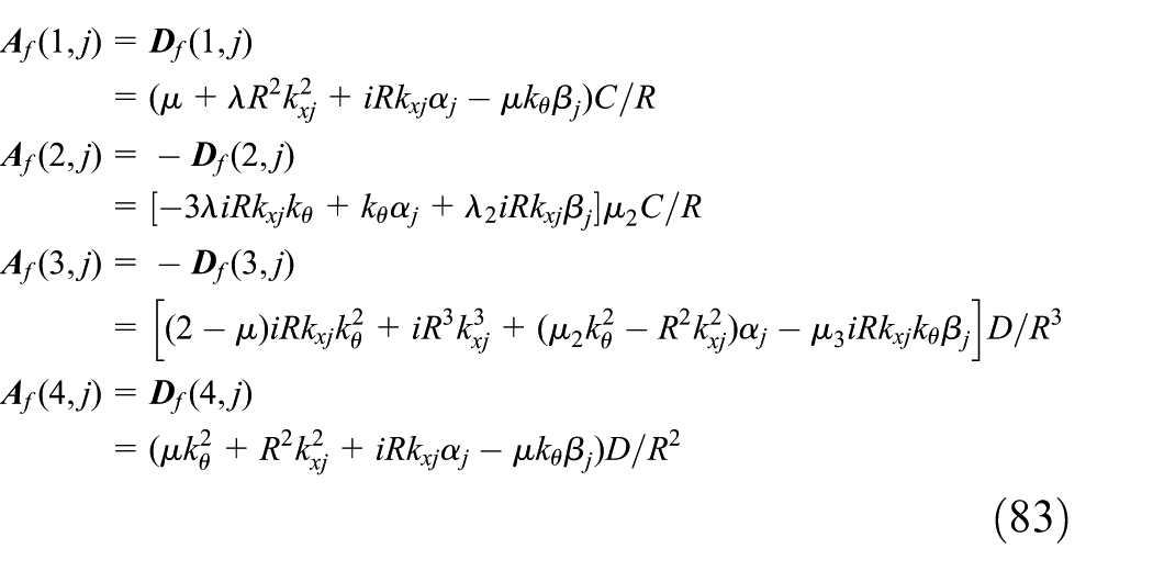
where j = 1, 2, 3, 4.

Equation of the natural frequencies

Taking advantage of the unidirectional traveling wave form solutions of the OCCS with SS curved edges and SS straight edges, respectively, obtained in sections “Solutions for the OCCS with the curved edges supported by SSs” and “Solutions for the OCCS with SS straight edges,” the MRRM is introduced to derive the equation of natural frequencies of the OCCS. Since the scattering matrix is related to the boundary conditions of the remaining two edges, it will be discussed in the first step. Then, the phase matrix and permutation matrix, which are independent of the boundary conditions, are obtained. Finally, the reverberation-ray matrix and the equation of natural frequencies of the OCCS are derived. The formulations mentioned above are presented in detail in the following discussion.

Since the derivation procedures for equations of natural frequencies of the OCCS with SS curved edges and SS straight edges are quite similar to each other, the one for SS curved edges will be taken as an example and the other one will be omitted. Note that the only difference between the two derivation procedures is that the one for SS curved edges takes advantage of the solutions obtained in section “Solutions for the OCCS with the curved edges supported by SSs” while the other one employs the solutions obtained in section “Solutions for the OCCS with SS straight edges” instead.

Scattering matrix for various classical boundary conditions

With regard to an OCCS with SS curved edges and SS straight edges, the boundary conditions and the dual local coordinate systems of the OCCS are, respectively, shown in Figure 3(a) and (b). The scattering matrices for the remaining two edges corresponding to various classical boundary conditions, including SS, FE, and clamped edge (CE), are derived in the following discussion.

Figure 3.

Boundary conditions and the dual local coordinate system of the shell: (a) curved edges supported by SSs and (b) straight edges supported by SSs.

1. SS

Assuming that the OCCS is SS at Node Line 1, namely, the boundary conditions are defined in the local coordinate (oxθz)¹² as

u^{12} = 0, w^{12} = 0, N_{θ θ}^{12} = 0, M_{θ θ}^{12} = 0

(84)

Substitution of equations (39), (41), (46), and (47) into the Fourier transform of equation (84) yields

\sum_{j = 1}^{4} α_{j} (a_{j}^{12} + d_{j}^{12}) = 0

(85)

\sum_{j = 1}^{4} (a_{j}^{12} + d_{j}^{12}) = 0

(86)

\sum_{j = 1}^{4} (λ_{1} - λ k_{θ j}^{2} - μ R k_{x} α_{j} + i k_{θ j} β_{j}) (a_{j}^{12} + d_{j}^{12}) = 0

(87)

\sum_{j = 1}^{4} (1 - k_{θ j}^{2} - μ R^{2} k_{x}^{2}) (a_{j}^{12} + d_{j}^{12}) = 0

(88)

Equations (85)–(88) can be presented in matrix form as

d^{1} = S^{1} a^{1}

(89)

where d ¹ = d ¹² = {d₁¹²d₂¹²d₃¹²d₄¹²}^T and a ¹ = a ¹² = {a₁¹²a₂¹²a₃¹²a₄¹²}^T are the amplitude vectors of the departing wave and the arriving wave, respectively, and S ¹ = − I ₄ is defined as the scattering matrix at Node Line 1, in which I ₄ is a unit matrix of fourth order.

2. FE

Assuming that the edge of the OCCS at Node Line 1 is free, namely, the boundary conditions are defined in the local coordinate (oxθz)¹² as

F_{θ x}^{12} = 0, N_{θ θ}^{12} = 0, V_{θ z}^{12} = 0, M_{θ θ}^{12} = 0

(90)

Substitution of equation (75) into the Fourier transform of equation (90) yields

W_{f}^{* 12} = A_{f} P_{h} (0) a^{12} + D_{f} P_{h} (0) d^{12} = 0

(91)

Since the phase matrix turns into a unit matrix at the origin of the local coordinate, equation (91) can be presented in the same form as equation (89) with the scattering matrix replaced by S ¹ = − D _f⁻¹ A _f.

3. CE

Assuming that the edge of the OCCS at Node Line 1 is clamped, namely, the boundary conditions are defined in the local coordinate (oxθz)¹² as

u^{12} = 0, v^{12} = 0, w^{12} = 0, ϕ_{θ}^{12} = 0

(92)

Substitution of equation (67) into the Fourier transform of equation (92) results in

W_{d}^{* 12} = A_{d} P_{h} (0) a^{12} + D_{d} P_{h} (0) d^{12} = 0

(93)

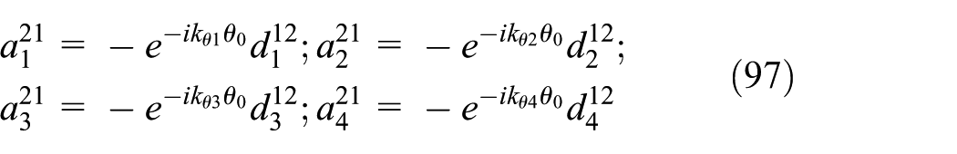
In a same manner, equation (93) can be presented in the same form as equation (89) with the scattering matrix replaced by S ¹ = − D _d⁻¹ A _d.

Similarly, the scattering relation for the OCCS at Node Line 2 is presented as

d^{2} = S^{2} a^{2}

(94)

where d ² = d ²¹ = {d₁²¹d₂²¹d₃²¹d₄²¹}^T and a ² = a ²¹ = {a₁²¹a₂²¹a₃²¹a₄²¹}^T are the amplitude vectors of the departing wave and the arriving wave at Node Line 2, respectively. In the same manner as the scattering matrix for Node Line 1 is derived, the scattering matrix at Node Line 2 is obtained as S ² = − I ₄ for an SS edge, S ² = − D _f⁻¹ A _f for an FE, and S ² = − D _d⁻¹ A _d for a CE.

Assembling both the local scattering equations at Node Line 1 and Node Line 2 by stacking d ¹, d ² and a ¹, a ² into two column vectors d and a , the global scattering equation is obtained

d = Sa

(95)

where d = {( d ¹)^T ( d ²)^T}^T and a = {( a ¹)^T ( a ²)^T}^T are the global amplitude vectors of the departing wave and the arriving wave, respectively, and S = diag{ S ¹ S ²} is the global scattering matrix.

Phase matrix and permutation matrix

The phase relations of harmonic waves in dual local coordinate system of MRRM provide additional equations for solving the unknown amplitude vectors. Note that the departing wave from Node Line 1 is exactly the arriving wave to Node Line 2, and vice versa. Therefore, the amplitudes of the departing wave and the arriving wave differ with each other by a phase factor.

With the employment of the solutions of the OCCS with SS curved edges, the relations between the amplitudes of the departing wave and the arriving wave are presented as

\begin{array}{l} a_{1}^{12} = - e^{- i k_{θ 1} θ_{0}} d_{1}^{21}; a_{2}^{12} = - e^{- i k_{θ 2} θ_{0}} d_{2}^{21}; \\ a_{3}^{12} = - e^{- i k_{θ 3} θ_{0}} d_{3}^{21}; a_{4}^{12} = - e^{- i k_{θ 4} θ_{0}} d_{4}^{21} \end{array}

(96)

\begin{array}{l} a_{1}^{21} = - e^{- i k_{θ 1} θ_{0}} d_{1}^{12}; a_{2}^{21} = - e^{- i k_{θ 2} θ_{0}} d_{2}^{12}; \\ a_{3}^{21} = - e^{- i k_{θ 3} θ_{0}} d_{3}^{12}; a_{4}^{21} = - e^{- i k_{θ 4} θ_{0}} d_{4}^{12} \end{array}

(97)

which are rewritten in matrix form as

a^{1} = - P_{h} (- θ_{0}) d^{2}

(98)

a^{2} = - P_{h} (- θ_{0}) d^{1}

(99)

Assembling both the local phase equations defined by equations (98) and (99) results in the global phase equation

a = P d^{*}

(100)

where a is defined in equation (95), while d ^* = {( d ²)^T ( d ¹)^T}^T is a rearranged global amplitude vector of the departing wave, and P = −diag{ P _h(−θ₀) P _h(−θ₀)} is the global phase matrix.

A comparison of the two global amplitude vectors of the departing wave d and d ^* indicates that the two amplitude vectors contain the same scalar state variables arranged in different sequential orders. The relation between d and d ^* is

d^{*} = Ud

(101)

where U = [ 0 ₄ I ₄; I ₄ 0 ₄] is the permutation matrix from d to d ^*, in which the block matrices 0 ₄ and I ₄ are, respectively, the zero matrix and the unit matrix of fourth order.

Equation of natural frequencies

Substitution of equations (100) and (101) into equation (95) yields

(I - R) d = 0

(102)

where R = SPU is defined as the reverberation-ray matrix.

To obtain a nontrivial solution of the global amplitude vector of the departing wave, the determinant of ( I − R ) must be 0, namely

det (I - R) = 0

(103)

which is the equation of natural frequencies of the OCCS.

Searching algorithm for natural frequencies

As the equation of natural frequencies of the OCCS is obtained, the problem at hand is to solve the equation for the natural frequencies. It is obvious that the left-hand side of equation (103) represents a function of frequency and the natural frequencies are zeros of the function. Unfortunately, for most values of the frequency, the left-hand side of equation (103) is complex numbers, which indicates that finding the zeros needs to search the common zeros of the real part and the imaginary part of the function. To address this problem, a good idea is to search the zeros or the minimal values of the absolute value of the function. This simple approach is adopted in this article and the golden section search algorithm is introduced to determine the natural frequencies of the OCCS. The procedure for determining natural frequencies of the OCCS is shown in Figure 4.⁶⁶

Figure 4.

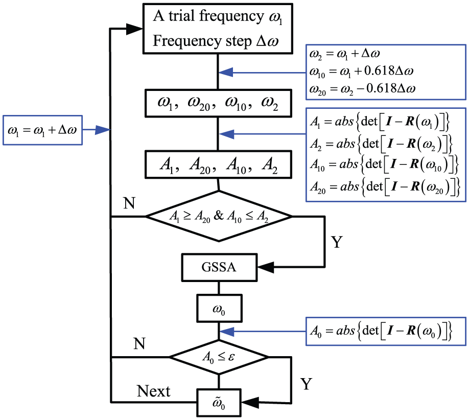
Procedure for determining natural frequencies of the OCCS.

It should be pointed out that since an increase in a frequency step Δω from the last natural frequency can be the initial estimation of the next natural frequency, only the initial estimation of the lowest natural frequency needs to be determined for a given circumferential mode number. The initial estimation of the lowest natural frequency can be determined from the curve of the absolute value of the determinant ( I − R ) against the frequency. The frequency step Δω is usually taken as a small number to avoid missing any possible values of the natural frequency. In this article, frequency step Δω is taken as 0.5 Hz, and the predefined tolerance ε is taken as 1 × 10⁻⁸.

Besides, a calculation example is presented here to clarify the efficiency of the golden section search algorithm compared with other methods; specifically, the dichotomy method is chosen as the comparison method. Both the methods are applied to calculate the natural frequency for mode number (m, n) = (1, 1) of the OCCS with the two curved edges SS and the two straight edges clamped. The initial estimation of the natural frequency and the frequency step are, respectively, taken as 6.5 and 0.6 Hz, which are consistent with the initial searching interval (6.5, 7.1) for the dichotomy method. The consuming time for the golden section search algorithm is 0.027439 s (obtained by tic-toc in MATLAB) to find the minimum or zero point for the absolute value, and the consuming time for the dichotomy method is 0.021495 s to find the zero point for the real part and 0.037846 s to find the zero point for the imaginary part. Therefore, it is more efficient to use the golden section search algorithm to find the roots for the natural frequency characteristic equation.

Mode shape calculation for the OCCS

Substituting one of the natural frequencies determined in the preceding section into equation (102), the global amplitude vector of the departing wave d is obtained. By normalization, the global amplitude vector of the departing wave is determinate. Subsequently, substituting the global amplitude vector of the departing wave into equations (100) and (101), the global amplitude vector of the arriving wave a is determined.

Finally, substituting the global amplitude vector of the departing wave and the arriving wave into the expressions of the displacement components of the OCCS, the mode shape corresponding to the given natural frequency is obtained.

Results and discussions

The MRRM and the golden section search algorithm are applied in this section to obtain the natural frequencies of the OCCS. To begin with, the method and the procedure presented in this article are verified by FEM and the results are given by other researchers. Then, the effects of different boundary conditions on the natural frequencies are examined.

Verification of this method

To verify the validity of the method for determining natural frequencies of the OCCS presented in the preceding sections, the natural frequencies of the OCCS with all four SS edges are obtained and the results are compared with those obtained by FEM and the method adopted by Leissa.¹ The basic parameters of the OCCS remain unchanged in this section and they are defined in Table 1.

Table 1.

Basic parameters of the OCCS.

Parameters	E (Pa)	µ	ρ (kg m⁻³)	h (m)	R (m)	L (m)	θ ₀
Value	2.1e11	0.3	7800	0.006	5	10	30°

The calculation results of the comparison study are presented in Table 2, in which the integer numbers m and n denote the half-wave numbers of the vibration modes in axial and circumferential directions, respectively. MRRM1 and MRRM2 represent the calculation results obtained by MRRM from the solutions for the OCCS with SS curved edges derived in section “Solutions for the OCCS with the curved edges supported by SSs” and the results obtained by MRRM from the solutions for the OCCS with SS straight edges derived in section “Solutions for the OCCS with SS straight edges.”

Table 2.

Comparison of natural frequencies (Hz) obtained by FEM, LM, and MRRM.

	Method	m = 1	m = 2	m = 3	m = 4	M = 5	m = 6	m = 7	m = 8
n = 1	FEM	10.704	34.971	62.339	85.755	103.823	117.321	127.288	134.768
	LM	10.670545	35.107418	62.313407	85.705677	103.792982	117.257758	127.236618	134.722961
	MRRM1	10.670545	35.107418	62.313407	85.705677	103.792982	117.257758	127.236618	134.722961
	MRRM2	10.670545	35.107418	62.313407	85.705677	103.792982	117.257758	127.236618	134.722961
n = 2	FEM	9.245	14.052	24.183	37.104	50.937	64.442	76.948	88.190
	LM	9.124489	13.956864	24.095000	37.042311	50.849047	64.322359	76.813398	88.048271
	MRRM1	9.124489	13.956864	24.095000	37.042311	50.849047	64.322359	76.813398	88.048271
	MRRM2	9.124489	13.956864	24.095000	37.042311	50.849047	64.322359	76.813398	88.048271
n = 3	FEM	19.712	20.693	23.368	28.291	35.164	43.364	52.293	61.447
	LM	19.529543	20.518652	23.216612	28.135055	35.009690	43.202241	52.098116	61.231057
	MRRM1	19.529543	20.518652	23.216612	28.135055	35.009690	43.202241	52.098116	61.231057
	MRRM2	19.529543	20.518652	23.216612	28.135055	35.009690	43.202241	52.098116	61.231057
n = 4	FEM	34.895	35.585	36.585	38.599	41.626	45.754	50.850	56.766
	LM	34.611327	35.156749	36.304889	38.308699	41.351241	45.473053	50.574066	56.468348
	MRRM1	34.611327	35.156749	36.304889	38.308699	41.351241	45.473053	50.574066	56.468348
	MRRM2	34.611327	35.156749	36.304889	38.308699	41.351241	45.473053	50.574066	56.468348
n = 5	FEM	54.536	55.015	55.846	57.172	59.042	61.516	64.666	68.463
	LM	54.038644	54.509184	55.361078	56.678222	58.547144	61.035810	64.178312	67.969398
	MRRM1	54.038644	54.509184	55.361078	56.678222	58.547144	61.035810	64.178312	67.969398
	MRRM2	54.038644	54.509184	55.361078	56.678222	58.547144	61.035810	64.178312	67.969398
n = 6	FEM	78.672	79.141	79.922	81.022	82.561	84.511	86.917	89.811
	LM	77.788236	78.240845	79.018718	80.152971	81.679598	83.633574	86.043356	88.926761
	MRRM1	77.788236	78.240845	79.018718	80.152971	81.679598	83.633574	86.043356	88.926761
	MRRM2	77.788236	78.240845	79.018718	80.152971	81.679598	83.633574	86.043356	88.926761
n = 7	FEM	107.366	107.859	108.614	109.685	111.097	112.822	114.959	117.468
	LM	105.856987	106.304171	107.059015	108.134587	109.546885	111.312922	113.448758	115.967731
	MRRM1	105.856987	106.304171	107.059015	108.134587	109.546885	111.312922	113.448758	115.967731
	MRRM2	105.856987	106.304171	107.059015	108.134587	109.546885	111.312922	113.448758	115.967731
N = 8	FEM	140.590	141.252	142.001	143.047	144.404	146.082	148.089	150.436
	LM	138.244285	138.689539	139.435974	140.489671	141.858332	143.550567	145.575129	147.940157
	MRRM1	138.244285	138.689539	139.435974	140.489671	141.858332	143.550567	145.575129	147.940157
	MRRM2	138.244285	138.689539	139.435974	140.489671	141.858332	143.550567	145.575129	147.940157

FEM: finite element method; LM: Leissa’s method; MRRM: method of reverberation-ray matrix.

It is observed from Table 2 that an excellent agreement is achieved between the results obtained by MRRM based on the two solutions and the results obtained by the method of Leissa. Therefore, the comparison study confirms the validity of MRRM for vibration analysis of OCCSs. Meanwhile, the results obtained by FEM are quite close to those obtained by the analytical methods and the mode shapes obtained by FEM and MRRM agree well with each other, which also indicates that the calculation results obtained by MRRM are validated.

Some mode shapes calculated by FEM and MRRM are presented in Figure 5. The FEM results are obtained with the common program software ANSYS, in which the geometric and material properties of the OCCS are defined according to Table 1, and 500 × 132 finite element mesh (element edge length 0.02 m) of SHELL181 elements is used during the calculation.

Figure 5.

Comparison of some selected mode shapes calculated by FEM and MRRM: (a) FEM (m, n) = (1, 1), (b) FEM (m, n) = (3, 2), (c) FEM (m, n) = (5, 2), (d) FEM (m, n) = (8, 3), (e) MRRM (m, n) = (1, 1), (f) MRRM (m, n) = (3, 2), (g) MRRM (m, n) = (5, 2) and (h) MRRM (m, n) = (8, 3).

Besides, this method is employed to calculate the natural frequencies of an OCCS with the geometric parameters such as shell length of 0.2 m, shell radius of 0.1 m, shell thickness of 0.001 m, and the included angle of π/3 and the material properties such as Young’s modulus E = 2.1 × 1011 Pa, Poisson’s ratio µ = 0.3, and mass density ρ = 7800 kg m⁻³. Comparison of the results obtained by this method and those given by other researchers is presented in Table 3.

Table 3.

Comparison of natural frequencies (Hz) of the OCCS having its two curved edges simply supported and two straight edges free.

(m, n)	Selmane and Lakis⁸	Ye et al.²⁷	Selmane and Lakis⁸		This method
(m, n)	Selmane and Lakis⁸	Ye et al.²⁷	Theory	Experiment	This method
(1, 1)	286	285.162	299	300	294.158504
(1, 2)	476	475.131	474	470	472.916461
(1, 3)	1486	1486.98	1530	1490	1483.169514
(2, 1)	859	857.365	860	870	884.978401
(2, 2)	819	817.600	840	850	849.578247
(3, 2)	1341	1339.58	1320	1330	1338.628360
(3, 3)	1440	1437.56	1450	1460	1434.462945

It can be observed from Table 3 that the present results are close to the results given by the other researchers. For most of the mode numbers, they are more close to the experimental results presented in Selmane and Lakis.⁸ This further proves the validation of the method presented in this article.

Results for the OCCS with SS curved edges

Having gained confidence in this method, it is subsequently employed to calculate natural frequencies of the OCCS with the two curved edges SS while the remaining two edges supported by an arbitrary combination of SS, CE, and FE based on the solutions derived in section “Solutions for the OCCS with the curved edges supported by SSs.” The basic parameters of the OCCS are defined in Table 1 and the calculation results corresponding to various boundary conditions of the remaining two edges are presented in Table 4. It should be pointed out that the FE effect is neglected in determining the mode number for each of the natural frequencies. As the remaining two edges are supported by SS–CE, CE–CE, and CE–FE, the natural frequencies corresponding to the circumferential mode number n = 1 are almost the same, which indicates that with two curved edges SS and one of the straight edges clamped, the boundary condition of the remaining edge hardly affects the natural frequencies of the OCCS corresponding to the circumferential mode number n = 1.

Table 4.

Natural frequencies (Hz) of the OCCS with the curved edges simply supported and the remaining two edges supported by various boundary conditions.

	BCs	m = 1	m = 2	m = 3	m = 4	m = 5	m = 6	m = 7	m = 8
n = 1	CE–CE	6.903722	13.891401	20.879705	27.868445	34.857583	41.847107	48.837011	55.827293
	SS–CE	6.903722	13.891401	20.879705	27.868445	34.857583	41.847107	48.837011	55.827293
	CE–FE	6.903722	13.891401	20.879705	27.868445	34.857583	41.847107	48.837011	55.827293
	SS–FE	7.258302	25.015109	48.319227	71.740337	91.883907	107.791848	119.919424	129.160567
	FE–FE	6.120653	18.220430	37.504015	58.897226	79.590906	97.235248	111.439212	122.487108
n = 2	CE–CE	20.523125	31.210487	37.734090	42.263241	46.947986	52.284187	58.251669	64.687323
	SS–CE	10.490254	17.504662	24.179185	30.588391	37.740488	44.823585	51.526802	58.200481
	CE–FE	18.549572	16.232324	23.701356	30.203734	36.896725	44.116670	51.376246	58.393447
	SS–FE	11.223650	13.891401	21.177688	32.215934	44.344305	57.587482	70.307903	81.606433
	FE–FE	13.695009	15.266162	19.990224	28.586345	39.518365	50.976221	63.783761	75.309691
n = 3	CE–CE	24.501907	26.756723	31.806439	38.848772	46.706796	54.441422	61.552789	68.048946
	SS–CE	21.219333	24.659882	33.133305	39.876810	45.112316	51.453948	58.796478	66.066847
	CE–FE	27.498331	26.477184	32.173507	40.865276	47.301419	52.752348	58.970906	66.009730
	SS–FE	22.920446	23.593212	25.698765	29.174879	34.684294	41.673208	49.679497	58.428579
	FE–FE	26.585686	27.378666	28.740059	31.579777	35.816470	41.527777	48.466439	56.239866
n = 4	CE–CE	44.928310	50.746539	62.307224	74.391611	83.018996	88.571267	92.855157	96.866365
	SS–CE	35.123599	38.789704	42.654966	51.601145	59.661057	64.577951	69.343500	74.981509
	CE–FE	43.950880	41.162437	44.728791	49.505511	58.261332	66.412407	72.058629	77.120674
	SS–FE	39.088652	39.658519	40.724381	42.524350	45.459682	48.585069	53.006155	58.022116
	FE–FE	43.834986	44.428358	45.514819	47.200740	49.605476	53.224780	56.367106	61.061256
n = 5	CE–CE	63.334581	64.057457	65.539474	67.932764	71.417444	76.138830	82.027109	88.688312
	SS–CE	60.538998	58.237123	60.477692	63.851767	71.161321	80.597777	87.623122	92.541903
	CE–FE	65.283672	67.936110	64.960395	67.879206	71.793301	78.524050	87.289900	95.162854
	SS–FE	59.592850	60.103195	61.003260	62.322064	64.167368	66.564351	69.228786	73.017729
	FE–FE	65.414608	65.963783	66.912725	68.326506	70.054298	72.43797802	75.317309	78.722657
n = 6	CE–CE	91.426878	92.663869	95.141839	99.664816	106.760979	115.040668	122.742891	129.285440
	SS–CE	84.660227	89.275055	84.110102	86.222443	88.834099	92.894699	99.334119	106.899746
	CE–FE	91.084812	92.307673	97.434267	91.674760	94.399931	97.303068	101.017933	106.036713
	SS–FE	84.418677	84.909402	85.744228	86.946412	88.509050	90.530319	92.969628	95.855445
	FE–FE	91.317643	91.843073	92.732108	93.997699	95.656947	97.725741	100.216799	103.137874
n = 7	CE–CE	119.568101	119.655372	120.455325	121.655320	123.239762	125.212056	127.572977	130.313495
	SS–CE	113.609849	114.726766	119.201246	113.583629	115.964385	118.291922	120.972048	124.124957
	CE–FE	121.065963	122.111689	123.614524	127.039067	121.677433	125.175760	128.073330	131.110768
	SS–FE	113.564593	114.045876	114.854974	116.001213	117.496047	119.352299	121.602554	124.166958
	FE–FE	121.541059	122.054372	122.914775	124.128739	125.703972	127.648519	129.970061	132.675902
n = 8	CE–CE	156.044110	156.570925	157.485610	158.765738	160.395829	162.348160	164.584677	165.385803
	SS–CE	147.011815	147.630298	148.755319	150.471182	152.816074	155.536973	158.213122	160.685088
	CE–FE	156.036760	156.528315	157.514014	158.910599	160.701222	162.814401	165.259246	167.660123
	SS–FE	147.029603	147.505224	148.301139	149.421588	150.871984	152.658238	154.786200	157.261119
	FE–FE	156.084009	156.588366	157.430801	158.614652	160.143151	162.020060	164.248910	166.832644

BC: boundary condition; CE: clamped edge; SS: simply supported; FE: free edge.

For a better illustration, the results presented in Table 4 are plotted in Figure 6, in which the variation curves of natural frequencies against the circumferential mode number are shown for each of the axial mode numbers.

Figure 6.

Comparison of natural frequencies of the OCCS with simply supported curved edges and the remaining two edges supported by various boundary conditions.

It can be observed from Figure 6 that for most axial mode numbers with an exception of m = 1, the natural frequencies for SS–SS, SS–FE, and FE–FE vary against the circumferential mode number in a similar pattern, which means that the natural frequencies of the OCCS first decrease and then increase with the increase in the circumferential mode number. The minimal natural frequency corresponds to different circumferential mode numbers for different axial mode numbers and different boundary conditions. In this article, the circumferential mode number corresponding to the minimal natural frequency is defined as the minimal frequency mode number. As the circumferential mode number is smaller than the minimal frequency mode number, the natural frequencies for SS–SS, SS–FE, and FE–FE decrease in turn. However, as the circumferential mode number is larger than the minimal frequency mode number, the highest to lowest order for the natural frequencies corresponding to the three boundary conditions turns to be FE–FE, SS–FE, and SS–SS.

Meanwhile, for circumferential mode numbers smaller than 5 or 6, the natural frequencies corresponding to SS–CE and CE–FE are very close to each other, and they are approximately linearly related to the circumferential mode number. While as the circumferential mode number is larger than 5 or 6, the natural frequency curve of SS–CE approaches to coincide with the one for SS–FE, and the natural frequency curve of CE–FE tends to coincide with the one for FE–FE.

Besides, the natural frequencies corresponding to CE–CE fluctuate upon those for SS–CE and CE–FE. Generally, for even circumferential mode numbers, the natural frequencies of CE–CE are much larger than those of SS–CE and CE–FE, while for odd circumferential mode numbers, they are very close to those of SS–CE and CE–FE.

Results for the OCCS with SS straight edges

Based on the solutions derived in section “Solutions for the OCCS with SS straight edges,” the MRRMs are employed to calculate the natural frequencies of the OCCS with the two straight edges SS while the remaining two edges supported by an arbitrary combination of SS, CE, and FE. The basic parameters of the OCCS are defined in Table 1 and the calculation results corresponding to various boundary conditions of the remaining two edges are presented in Table 5.

Table 5.

Natural frequencies (Hz) of the OCCS with the straight edges simply supported and the remaining two edges supported by various boundary conditions.

	BCs	m = 1	m = 2	m = 3	m = 4	m = 5	m = 6	m = 7	m = 8
n = 1	CE–CE	23.124388	51.410851	77.986928	98.681822	113.953220	125.081184	133.307607	139.515363
	SS–CE	16.216781	43.088345	70.213646	92.377383	109.059520	121.329035	130.394052	137.210944
	CE–FE	23.145856	51.452118	78.001279	98.642080	113.858457	124.941952	133.134982	139.318156
	SS–FE	16.230300	43.126831	70.240390	92.357369	108.984778	121.206983	130.235575	137.025444
	FE–FE	23.167352	51.493407	78.015548	98.602656	113.764603	124.804499	132.964831	139.124303
n = 2	CE–CE	10.753030	18.740014	31.017625	45.020291	59.117438	72.370431	84.344311	94.925373
	SS–CE	9.733082	16.153963	27.427785	40.958483	54.955225	68.351950	80.606472	91.526786
	CE–FE	10.751662	18.731977	30.999115	44.990524	59.077875	72.323784	84.293800	94.874275
	SS–FE	9.732449	16.148223	27.412525	40.932233	54.918856	68.307757	80.557427	91.476047
	FE–FE	10.750295	18.723952	30.980632	44.960802	59.038368	72.277195	84.243337	94.823202
n = 3	CE–CE	19.733541	21.442630	25.310773	31.437934	39.261379	48.082755	57.330638	66.601835
	SS–CE	19.609820	20.919900	24.179345	29.706008	37.071814	45.597274	54.685717	63.901580
	CE–FE	19.733724	21.443076	25.310702	31.436231	39.257813	48.078398	57.327649	66.603084
	SS–FE	19.609942	20.920309	24.179505	29.704803	37.068723	45.593002	54.682105	63.901266
	FE–FE	19.733907	21.443522	25.310630	31.434530	39.254249	48.074041	57.324659	66.604335
n = 4	CE–CE	34.670464	35.410933	36.914179	39.417870	43.041713	47.744949	53.363346	59.677769
	SS–CE	34.637517	35.271568	36.585904	38.829804	42.157691	46.570072	51.933485	58.043605
	CE–FE	34.671043	35.413599	36.921132	39.431710	43.064948	47.779752	53.411652	59.741500
	SS–FE	34.637971	35.273729	36.591741	38.841802	42.178365	46.601648	51.977924	58.102807
	FE–FE	34.671623	35.416276	36.928111	39.445601	43.088266	47.814682	53.460147	59.805505
n = 5	CE–CE	54.066076	54.621275	55.619644	57.146433	59.281834	62.078982	65.551517	69.672797
	SS–CE	54.051510	54.561960	55.483498	56.901326	58.899543	61.539361	64.845053	68.800763
	CE–FE	54.067111	54.625645	55.630226	57.166748	59.315844	62.130741	65.624834	69.771033
	SS–FE	54.052420	54.565826	55.492939	56.919631	58.930519	61.587001	64.913199	68.892869
	FE–FE	54.068155	54.630054	55.640904	57.187248	59.350164	62.182967	65.698811	69.870155
n = 6	CE–CE	77.803931	78.303908	79.161361	80.407452	82.076868	84.201368	86.804233	89.896602
	SS–CE	77.795790	78.271231	79.087567	80.276073	81.872264	83.909698	86.414419	89.401040
	CE–FE	77.805361	78.309736	79.174845	80.432225	82.116909	84.260871	86.887411	90.007488
	SS–FE	77.797115	78.276639	79.100112	80.299198	81.909790	83.965707	86.493072	89.506378
	FE–FE	77.806810	78.315641	79.188507	80.457327	82.157482	84.321161	86.971679	90.119809
n = 7	CE–CE	105.867167	106.344882	107.150539	108.296938	109.799441	111.673913	113.934672	116.592741
	SS–CE	105.861951	106.324029	107.103689	108.213903	109.670402	111.489685	113.687003	116.274596
	CE–FE	105.868816	106.351524	107.165635	108.324111	109.842476	111.736711	114.021170	116.706808
	SS–FE	105.863519	106.330349	107.118067	108.239819	109.711516	111.549797	113.769979	116.384266
	FE–FE	105.870492	106.358271	107.180967	108.351708	109.886180	111.800479	114.108988	116.822589
n = 8	CE–CE	138.251546	138.718550	139.501105	140.605067	142.037761	143.807235	145.921464	148.387589
	SS–CE	138.247850	138.703787	139.467971	140.546385	141.946560	143.676849	145.745638	148.160592
	CE–FE	138.253259	138.725418	139.516607	140.632736	142.081180	143.870016	146.007211	148.499849
	SS–FE	138.249503	138.710413	139.482934	140.573109	141.988530	143.737592	145.828691	148.269454
	FE–FE	138.255001	138.732400	139.532366	140.660861	142.125308	143.933811	146.094325	148.613871

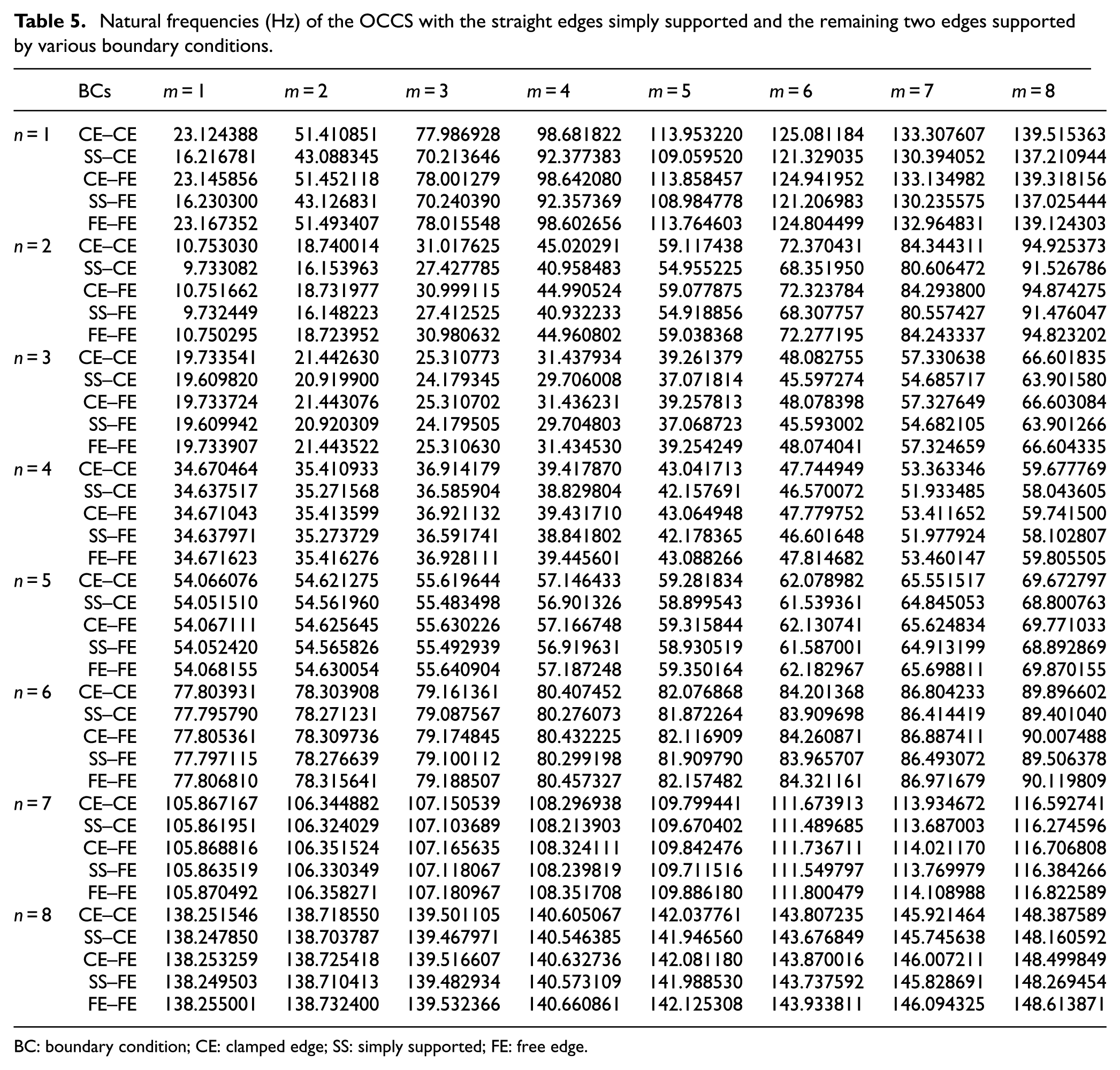
BC: boundary condition; CE: clamped edge; SS: simply supported; FE: free edge.

For a better illustration, the results presented in Table 5 are plotted in Figure 7, in which the variation curves of the natural frequencies against the axial mode number are shown for each of the circumferential mode numbers.

Figure 7.

Comparison of natural frequencies of the OCCS with simply supported straight edges and the remaining two edges supported by various boundary conditions.

It can be observed from Figure 7 that with the two straight edges SS, the effects of boundary conditions of the remaining two edges on the natural frequencies of the OCCS are not significant in general. The natural frequencies for FE–FE, CE–FE, CE–CE, SS–FE, SS–CE, and SS–SS decrease in sequence.

Figure 7 also shows that for circumferential mode numbers smaller than 6, the natural frequencies of the OCCS for different boundary conditions vary with the axial mode number in three different curves. Specifically, CE–CE, CE–FE, and FE–FE share the highest one, SS–CE and SS–FE take the middle one, and SS–SS holds the lowest one. However, as the circumferential mode number is larger than 6, all the natural frequencies corresponding to various boundary conditions are very close to each other, which indicates that for large circumferential mode numbers, boundary conditions of the curved edges have no much influence on the natural frequencies of the OCCS with the two straight edges SS.

Conclusion

This article presents an analytical solution procedure for free vibration analysis of the OCCS with two opposite edges SS and the remaining two edges supported by various combinations of classical boundary conditions. Based on the Flügge thin shell theory, the force and moment resultants and the equations of motion for an OCCS are introduced. With the employment of Fourier transform, the solutions of the traveling wave form along the SS edges and the standing wave form along the remaining two edges are obtained. Then, MRRM is applied to derive the equation of natural frequencies and the golden section search algorithm is employed to solve for the natural frequencies of the OCCS. The proposed method has been verified through the comparison of the present results against those obtained by FEM and presented in available literature. Finally, the effects of boundary conditions of the remaining two edges on the natural frequencies are investigated. It can be concluded as follows:

With the two curved edges SS and one of the straight edges clamped, the boundary condition of the remaining edge hardly affects the natural frequencies of the OCCS corresponding to the circumferential mode number n = 1.

With the two curved edges SS, the natural frequencies for SS–SS, SS–FE, and FE–FE vary against the circumferential mode number in a similar pattern, namely, first decrease and then increase with the increase in the circumferential mode number for most axial mode numbers. The natural frequencies corresponding to SS–CE and CE–FE are very close to each other for small circumferential mode numbers; however, the natural frequency curve of SS–CE tends to coincide with the one for SS–FE, and the natural frequency curve of CE–FE tends to coincide with the one for FE–FE for large circumferential mode numbers.

With the two straight edges SS, the effects of boundary conditions of the remaining two edges on the natural frequencies of the OCCS are not significant in general. However, the natural frequencies for FE–FE, CE–FE, CE–CE, SS–FE, SS–CE, and SS–SS decrease in sequence.

For small circumferential mode numbers, the natural frequencies of the OCCS for different boundary conditions vary with the axial mode number in three different curves, CE–CE, CE–FE, and FE–FE share the highest one, SS–CE and SS–FE take the middle one, and SS–SS holds the lowest one. However, for large circumferential mode numbers, boundary conditions of the curved edges have no much influence on the natural frequencies of the OCCS with the two straight edges SS.

It is particularly pointed out that the formulation presented in this article is a fundamental work to apply MRRM to vibration analysis of complex structures composed of OCCSs.

Footnotes

Appendix 1

For simplicity and clarity of this article, some lengthy linear differential operators and parameters are replaced by equivalent indexes. However, for the strictness of the presentation, the equivalent indexes are defined in the appendix.

Acknowledgements

The authors would like to sincerely thank Miss Jingjing Yu and Mr Qingshan Wang for the scientific discussions and suggestions and the anonymous reviewers for the critical and constructive comments on this article.

Academic Editor: Farzad Ebrahimi

Declaration of conflicting interests

The author(s) declared no potential conflicts of interest with respect to the research, authorship, and/or publication of this article.

Funding

The author(s) disclosed receipt of the following financial support for the research, authorship, and/or publication of this article: This work was financially supported by National Natural Science Foundation of China (Grant Nos 51509047, 51279038, and 51479041) and Fundamental Research Funds for Central Universities (HEUCF150105). The authors would like to express their profound thanks for the financial support.

References

Leissa

AW.

Vibration of shells. Washington, DC: Scientific and Technical Information Office, National Aeronautics and Space Administration, 1973, pp.5–175.

Sewall

JL.

Vibration analysis of cylindrically curved panels with simply supported or clamped edges and comparison with some experiments. Washington, DC: Langley Research Center, National Aeronautics and Space Administration, 1967.

Leissa

Lee

Wang

AJ.

Vibrations of cantilevered shallow cylindrical shells of rectangular planform. J Sound Vib 1981; 78: 311–328.

Leissa

Narita

Vibrations of completely free shallow shells of rectangular planform. J Sound Vib 1984; 96: 207–218.

Cheung

Tham

LG.

Free vibration analysis of singly curved shell by spline finite strip method. J Sound Vib 1989; 128: 411–422.

Chakravorty

Bandyopadhyay

JN.

On the free vibration of shallow shells. J Sound Vib 1995; 185: 673–684.

Bardell

Dunsdon

Langley

RS.

On the free vibration of completely free, open, cylindrically curved isotropic shell panels. J Sound Vib 1997; 207: 647–669.

Selmane

Lakis

AA.

Dynamic analysis of anisotropic open cylindrical shells. Comput Struct 1997; 62: 1–12.

Selmane

Lakis

AA.

Vibration analysis of anisotropic open cylindrical shells subjected to a flowing fluid. J Fluid Struct 1997; 11: 111–134.

10.

Nayak

Bandyopadhyay

JN.

On the free vibration of stiffened shallow shells. J Sound Vib 2002; 255: 357–382.

11.

Ohga

Takao

Shigematsu

Natural frequencies and modes of open cylindrical shells with a circumferential thickness taper. J Sound Vib 1995; 183: 143–156.

12.

Lim

Liew

KM.

A higher order theory for vibration of shear deformable cylindrical shallow shells. Int J Mech Sci 1995; 37: 277–295.

13.

Lim

Liew

Kitipornchai

Vibration of open cylindrical shells: a three-dimensional elasticity approach. J Acoust Soc Am 1998; 104: 1436–1443.

14.

Cleghorn

Fenton

RG.

On the accurate analysis of free vibration of open circular cylindrical shells. J Sound Vib 1995; 188: 315–336.

15.

Price

Liu

Taylor

. Vibrations of cylindrical pipes and open shells. J Sound Vib 1998; 218: 361–387.

16.

Zhang

Liu

Lam

KY.

Frequency analysis of cylindrical panels using a wave propagation approach. Appl Acoust 2001; 62: 527–543.

17.

Toorani

Lakis

AA.

Shear deformation in dynamic analysis of anisotropic laminated open cylindrical shells filled with or subjected to a flowing fluid. Comput Methods Appl M 2001; 190: 4929–4966.

18.

Gulgazaryan

GR.

Vibrations of a semi-infinite, orthotropic, cylindrical shell of open profile. Int Appl Mech 2004; 40: 199–212.

19.

Singh

Shen

LB.

Free vibration of open circular cylindrical composite shells with point supports. J Aerospace Eng 2005; 18: 120–128.

20.

Kandasamy

Singh

AV.

Free vibration analysis of skewed open circular cylindrical shells. J Sound Vib 2006; 290: 1100–1118.

21.

Zhang

Xiang

Vibration of open circular cylindrical shells with intermediate ring supports. Int J Solids Struct 2006; 43: 3705–3722.

22.

Zhang

Xiang

Vibration of open cylindrical shells with stepped thickness variations. J Eng Mech: ASCE 2006; 132: 780–784.

23.

Gulgazaryan

Saakyan

RD.

The vibrations of a thin elastic orthotropic circular cylindrical shell with free and hinged edges. J Appl Math Mech 2008; 72: 312–322.

24.

Kandasamy

Singh

AV.

Free vibration analysis of cylindrical shells supported on parts of the edges. J Aerospace Eng 2009; 23: 34–43.

25.

Wang

Guo

Chang

. Nonlinear dynamic response of rotating circular cylindrical shells with precession of vibrating shape—part I: numerical solution. Int J Mech Sci 2010; 52: 1217–1224.

26.

Wang

Guo

Chang

. Nonlinear dynamic response of rotating circular cylindrical shells with precession of vibrating shape—part II: approximate analytical solution. Int J Mech Sci 2010; 52: 1208–1216.

27.

Jin

Chen

. A unified formulation for vibration analysis of open shells with arbitrary boundary conditions. Int J Mech Sci 2014; 81: 42–59.

28.

Jin

. A unified Chebyshev–Ritz formulation for vibration analysis of composite laminated deep open shells with arbitrary boundary conditions. Arch Appl Mech 2014; 84: 441–471.

29.

Jin

TG.

Free vibration analysis of moderately thick functionally graded open shells with general boundary conditions. Compos Struct 2014; 117: 169–186.

30.

Howard

Pao

YH.

Analysis and experiments on stress waves in planar trusses. J Eng Mech: ASCE 1998; 124: 884–891.

31.

Pao

Keh

Howard

SM.

Dynamic response and wave propagation in plane trusses and frames. AIAA J 1999; 37: 594–603.

32.

Pao

Sun

Dynamic bending strains in planar trusses with pinned or rigid joints. J Eng Mech: ASCE 2003; 129: 324–332.

33.

Pao

Tian

JY.

Reverberation matrix method for propagation of sound in a multilayered liquid. J Sound Vib 2000; 230: 743–760.

34.

Tian

Pao

YH.

Application of the reverberation-ray matrix to the propagation of elastic waves in a layered solid. Int J Solids Struct 2002; 39: 5447–5463.

35.

Tian

Yang

XY.

Transient elastic waves in a transversely isotropic laminate impacted by axisymmetric load. J Sound Vib 2006; 289: 94–108.

36.

Guo

Chen

WQ.

On free wave propagation in anisotropic layered media. Acta Mech Solida Sin 2008; 21: 500–506.

37.

Tian

Xie

ZM.

A hybrid method for transient wave propagation in a multilayered solid. J Sound Vib 2009; 325: 161–173.

38.

Tian

JY.

Generalized reverberation matrix formulation for wave propagation in multilayered medium. Acta Mech Solida Sin 2010; 23: 189–199.

39.

Tian

XY.

Crack detection in beams by wavelet analysis of transient flexural waves. J Sound Vib 2003; 261: 715–727.

40.

Chen

Mao

Sun

GJ.

The effects of damping on the transient response of frames using the method of reverberation ray matrix. J Shang Jiaot Univ 2005; 39: 154–156.

41.

Liu

Miao

Sun

GJ.

Modal analysis of frames with reverberation ray matrix method. J Vib Measure Diagnos 2006; 26: 322–323.

42.

YY.

Stress wave propagation and study on influencing factor in frame structure embedded partially in soil. Chin J Comput Mech 2007; 24: 659–663.

43.

YY.

Studies on wave responses of a defective frame structure embedded partially in soil and influence factors. J Vib Eng 2007; 20: 194–199.

44.

Guo

Chen

Pao

YH.

Dynamic analysis of space frames: the method of reverberation-ray matrix and the orthogonality of normal modes. J Sound Vib 2008; 317: 716–738.

45.

Jiang

Chen

WQ.

Reverberation-ray analysis of moving or distributive loads on a non-uniform elastic bar. J Sound Vib 2009; 319: 320–334.

46.

Miao

Sun

Pao

YH.

Vibration mode analysis of frames by the method of reverberation ray matrix. J Vib Acoust 2009; 131: 0510051–0510055.

47.

Jiang

JQ.

Transient responses of Timoshenko beams subject to a moving mass. J Vib Control 2011; 17: 1975–1982.

48.

Jiang

Chen

Pao

YH.

Reverberation-ray analysis of continuous Timoshenko beams subject to moving loads. J Vib Control 2011; 18: 774–784.

49.

Zhu

Xiang

. Dynamic behavior of cable-stayed beam with localized damage. J Vib Control 2011; 17: 1080–1089.

50.

Miao

Sun

Chen

KF.

Transient response analysis of balanced laminated composite beams by the method of reverberation-ray matrix. Int J Mech Sci 2013; 77: 121–129.

51.

Guo

Fang

DN.

Analysis and interpretation of longitudinal waves in periodic multiphase rods using the method of reverberation-ray matrix combined with the Floquet–Bloch theorem. J Vib Acoust 2014; 136: 0110061–01100613.

52.

Liu

Fang

. Active control of power flow transmission in finite connected plate. J Sound Vib 2010; 329: 4124–4135.

53.

Liu

Huang

WH.

Active vibration control of finite L-shaped beam with travelling wave approach. Acta Mech Solida Sin 2010; 23: 377–385.

54.

Zhu

Xiang

. Recursive formulae for wave propagation analysis of FGM elastic plates via reverberation-ray matrix method. Compos Struct 2011; 93: 259–270.

55.

Liu

Shen

. Application of the method of reverberation ray matrix to the early short time transient responses of stiffened laminated composite plates. J Appl Mech 2012; 79: 0410091–04100910.

56.

Zhu

Chen

GR.

Reverberation-ray matrix analysis for wave propagation in multiferroic plates with imperfect interfacial bonding. Ultrasonics 2012; 52: 125–132.

57.

Tian

XY.

Transient axisymmetric elastic waves in finite orthotropic cylindrical shells. Acta Sci Nat: Univ Pekin 2000; 36: 365–372.

58.

Liu

Huang

WH.

Transient wave propagation and early short time transient responses of laminated composite cylindrical shells. Compos Struct 2011; 93: 2587–2597.

59.

Liu

Chen

. Transient wave propagation in the ring stiffened laminated composite cylindrical shells using the method of reverberation ray matrix. J Acoust Soc Am 2013; 133: 770–780.

60.

Chen

Guo

YQ.

Modeling of FGM-TFBARS with the method of reverberation-ray matrix. In: Fan

Chen

(eds) Advances in heterogeneous material mechanics. Lancaster, PA: DEStech Publications, 2008, pp.1626–1630.

61.

Zhou

Chen

. Reverberation-ray matrix analysis of free vibration of piezoelectric laminates. J Sound Vib 2009; 326: 821–836.

62.

Miao

Sun

Chen

. Reverberation-ray matrix analysis of the transient dynamic responses of asymmetrically laminated composite beams based on the first-order shear deformation theory. Compos Struct 2015; 119: 394–411.

63.

Press

Teukolsky

Vetterling

. Numerical recipies in C: the art of scientific computing. 2nd ed.Cambridge: Cambridge University Press, 1992, pp.397–401.

64.

Vajda

Fibonacci and Lucas numbers, and the golden section: theory and applications. New York: Dover Publications, 2007.

65.

Flügge

Stresses in shell. Berlin: Springer, 1973.

66.

Guo

YQ.

The method of reverberation-ray matrix and its applications. PhD Thesis, Zhejiang University, Hangzhou, China, 2008, p.59.

Free vibration analysis of open circular cylindrical shells by the method of reverberation-ray matrix

Abstract

Keywords

Introduction

Formulation

Force and moment resultants

Governing differential equations

Solutions for the OCCS with the curved edges supported by SSs

Solutions for the OCCS with SS straight edges

Solutions expressed in matrix form

SS curved edges

SS straight edges

Equation of the natural frequencies

Scattering matrix for various classical boundary conditions

Phase matrix and permutation matrix

Equation of natural frequencies

Searching algorithm for natural frequencies

Mode shape calculation for the OCCS

Results and discussions

Verification of this method

Results for the OCCS with SS curved edges

Results for the OCCS with SS straight edges

Conclusion

Footnotes

Appendix 1

Acknowledgements

Declaration of conflicting interests

Funding

References