
Abstract
An emergency collision-preventing model is proposed for two vehicles driving from opposite directions. To study the impact of drivers’ strategies on traffic safety in this model, the relevant knowledge of game theory has been introduced. Based on the drivers’ strategies and payoff of every strategy, a game tree and a payoff matrix have been constructed. Mathematical method is applied to identify the pure-strategy Nash equilibrium and the mixed strategies Nash equilibrium. The occurrence probability of accidents under the Nash equilibrium is discussed here. The results suggest that under the pure-strategy Nash equilibrium, one driver must swerve. Furthermore, the probability of keeping original route is greater when drivers adopt the mixed strategies Nash equilibrium. The results presented in this article will provide some reference for drivers under similar conditions.
Introduction
With the increasing number of vehicles traveling on the road, the traffic accidents are also soaring. Among all traffic accidents, those caused by drivers’ decision on collision-preventing cannot be ignored. When driving the vehicles on secondary or below roads without the central reserves, some drivers do not observe the traffic rules. Then if an oncoming vehicle appears suddenly, the diver will easily make a wrong decision in panic, which often leads to an accident. Data show that straight vehicle accidents accounted for about 30% of all accidents happening in urban areas’ non-main intersections and outlying suburbs due to the absence of the traffic lights. 1 Such incidents are usually disastrous.
For two vehicles toward each other from opposite ends, the strategy the drivers take at the last moment remains uncertain as they intend to prevent collision. What we can get is the probability distribution of the established strategies. This increases the uncertainty of making collision-preventing decision. 2 Game theory has been used to analyze the problems in transportation areas, such as lane-changing, individual travel route choice, and speeding driving behavior.3–5 Therefore, the knowledge of game theory is introduced to explore drivers’ collision-preventing decisions.
Model description
Description for two vehicles game
In the real driving environment, driver A and driver B are required to pass through the point of conflict in a safe way and keep their present speed and driving space at the same time. Each driver will take into account the other’s possible choice of strategy when he selects his own one. For instance, if driver A turns left, as long as the driver B does not adopt the same strategy, it will not cause an accident. The original driving behaviors for both drivers will not be adjusted too much.
Game model
First, the roads involved in the research are defined as main highways without signal lamp or with less divided centerline, which are distributed in mountainous areas and towns. However, the effects of trees and other objects on the sides of the road for making collision-preventing decision are not taken into account. It is assumed that only the related vehicles’ information affects drivers’ strategy and that the repeated preventing collisions are not concerned. A typical scene involved in this article is the process of preventing collision of two vehicles. As is shown in Figure 1, driver A and driver B are moving ahead for a single lane from opposite directions.

Diagram of two vehicles driving from opposite directions.
Strategy of collision-preventing
Collision-preventing is an integrated process during which the drivers adjust strategies and realize their driving goals in accordance with their own driving characteristics, related vehicles’ speed, driving space, and any other information of the surroundings.
As is shown in Figure 1, according to driver A’s current speed, the current route, and the distance from driver B, the driver A estimates that two cars will have a collision (or scratch) and then considers to take a collision-preventing strategy.
In real driving environment, if drivers believe that the above situation will occur, they will slow down, definitely. Based on the drivers’ actions in real driving surroundings, this game involves three possible strategies, swerving on the left, swerving on the right, and staying straight while slowing down the speed. In the latter part, L, R, and M are used to represent three strategies, respectively.
Game tree and payoff matrix
This game consists of the following elements, players set, strategies set, game tree, and Nash equilibrium: 3
Player set. N = {1, 2}. N stands for player collections. Element in the set N is called as player or participant.
Strategy set. A player’s strategy set defines the strategies available for them. For instance, each player has the finite strategy set {swerving on the left, swerving on the right, staying straight while slowing down the speed} in this game.
Game tree. A game tree is a directed graph in which the nodes represent positions in a game and the edges mean moves. For a finite game, it can be represented by a game tree. 6
Nash equilibrium. The Nash equilibrium is a solution concept of a non-cooperative game involving two or more players, in which each player is assumed to know the equilibrium strategies of the others, and a player has nothing to gain by only changing his or her own strategy. 7
The game tree for this game is shown in Figure 2 (The payoffs in our model are related to drivers’ losses, such as time, speed, and economic losses. Because the specific weight values need investigation, we used algebraic expressions.)

Game tree.
From the game tree, one can see clearly that there are two drivers A and B. The numbers by every non-terminal node indicate to which player that decision node belongs. The numbers by every terminal node represent the payoffs to the players (e.g. (a11, b11) represents the payoff of a11 to driver A for taking L and the payoff of b11 to driver B for taking L). The labels by every edge of the graph are the name of the action that edge represents.
According to the game tree, this collision-preventing game can be shown in the following payoff matrix (Table 1).
Payoff matrix.
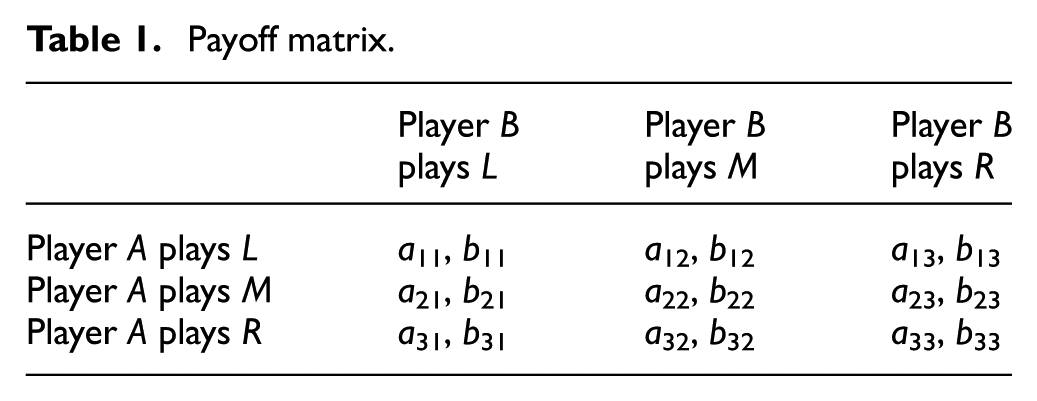
In Table 1, a11 = a12 = a32 = a33 = b11 = b21 = b23 = b33 = γ1, a21 = a33 = b12 = b32 = γ2, a13 = a22 = a31 = b13 = b22 = b31 = γ3, and γ2 > γ1 ≥ 0 > γ3, |γ3| > |γ2| > |γ1|. In Table 1, one can observe some information, like players, strategies, and payoffs. In the matrix, the first number is the payoff received by the row player (Player A in our example); the second is the payoff for the column player (Player B in our example).
Calculation and discussion
All anti-coordination games have three Nash equilibria. Two of these are pure contingent strategy profiles, in which each player plays one of the pair of strategies, and the other player chooses the opposite strategy. The third one is a mixed equilibrium, in which each player probabilistically chooses between the two pure strategies.
Pure-strategy Nash equilibrium
There is an easy numerical way to identify Nash equilibrium on a payoff matrix. The rule goes as follows: if the first payoff number, in the payoff pair of the cell, is the maximum of the column of the cell and if the second number is the maximum of the row of the cell, then the cell represents a Nash equilibrium.
Using the rule, we can see that the Nash equilibrium cells are (L, M), (M, L), (M, R), and (R, M). It means in this case, the pure-strategy equilibria are the four situations wherein one player swerves while the other does not.
The probability of an accident: in this case, both drivers choose to drive either on the left or on the right, there is no intersection set existing as for both drivers’ choice of strategy. Thus, the probability for an accident is zero.
Mixed strategies Nash equilibrium
The best response mapping for all 2 × 2 anti-coordination games is shown in Figure 3 (for our game, we can define the L and R as “swerving” temporarily). The variables x and y in Figure 3 are the probabilities of playing the escalated strategy (“Don’t swerve”) for players A and B, respectively. The line in graph on the left shows the optimum probability of playing the escalated strategy for player B as a function of x. The line in the second graph shows the optimum probability of playing the escalated strategy for player A as a function of y (the axes have not been rotated, so the dependent variable is plotted on the abscissa, and the independent variable is plotted on the ordinate). The Nash equilibria are where the players’ correspondences agree, that is, cross. These are shown with points in the right-hand graph. The best response mappings agree (i.e. cross) at three points. The first two Nash equilibria are in the top left and bottom right corners, where one player chooses one strategy, the other player chooses the opposite strategy. The third Nash equilibrium is a mixed strategy which lies along the diagonal from the bottom left to top right corners.

Best response mapping and Nash equilibria.
In order for a player to be willing to randomize, his expected payoff for each strategy should be the same. In addition, the sum of the probabilities for each strategy of a particular player should be 1 (Table 2). This creates a system of equations from which the probabilities of choosing each strategy can be derived. 8
Strategy probability.

In the collision-preventing game, to compute the mixed-strategy Nash equilibrium, it is feasible to assign A the probability p of playing L, t of playing M, and q of playing R and assign B the probability x of playing L, y of playing M, and z of playing R.
Expected payoff for A


In addition

So

In the same way, expected payoff for B


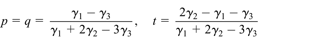
where
Thus, a mixed-strategy Nash equilibrium, in this game, is for each player to randomly choose L, M, or R with above probabilities.
Probability for an accident: since driver A or B randomly chooses his or her strategy, they may have the same choice. And the probability of taking L, M, or R is greater than zero, so it will cause an accident. The probability of an accident is connected to the payoff of each strategy.
Because the loss of swerving is so trivial compared to the crash that will occur if nobody swerves, to swerve seems to be the reasonable strategy.
Conclusion
An emergency collision-preventing model is proposed. By analyzing the drivers’ strategies based on game theory, the obtained conclusions are as follows:
Under the pure-strategy equilibrium, once one player swerves, the other one will never do the same choice. In this case, there is no accident.
Under the mixed strategies equilibrium, a driver chooses his or her strategy with a certain probability. And they prefer to not change his or her original route. Under this equilibrium, there could be an accident. The probability of an accident is connected to the payoff of each strategy.
Footnotes
Academic Editor: Geert Wets
Declaration of conflicting interests
The author(s) declared no potential conflicts of interest with respect to the research, authorship, and/or publication of this article.
Funding
The author(s) received no financial support for the research, authorship, and/or publication of this article.