Sage Journals: Discover world-class research

Abstract

Abnormal breast can be diagnosed using the digital mammography. Traditional manual interpretation method cannot yield high accuracy. In this study, we proposed a novel computer-aided diagnosis system for detecting abnormal breasts. Our dataset contains 200 mammogram images with size of 1024 × 1024. First, we segmented the region of interest from mammogram images. Second, the fractional Fourier transform was employed to obtain the unified time–frequency spectrum. Third, spectrum coefficients were reduced by principal component analysis. Finally, both support vector machine and k-nearest neighbors were used and compared. The proposed “weighted-type fractional Fourier transform+principal component analysis+support vector machine” achieved sensitivity of 92.22% ± 4.16%, specificity of 92.10% ± 2.75%, and accuracy of 92.16% ± 3.60%. It is better than both the proposed “weighted-type fractional Fourier transform+principal component analysis+k-nearest neighbors” and other five state-of-the-art approaches in terms of sensitivity, specificity, and accuracy. The proposed computer-aided diagnosis system is effective in detecting abnormal breasts.

Keywords

Fractional Fourier transform abnormal breast computer-aided diagnosis mammogram support vector machine

Background

Breast cancer is a common disease among women.¹ Digital mammogram (DM) is one of the most effective approaches for its early and accurate detection.² However, the manual interpretation procedure is hard for physicians.³ The reasons stem from (1) the complicated anatomic structure of the breast and (2) the similarity of the breast tissues (such as the dense breast) with cancer masses.

This motivated the necessity of developing computer-aided diagnosis (CAD) system.^4,5 Roughly, three different aims exist. First is to detect abnormal breasts from mammography. Second is to detect masses. Third is to distinguish malignant masses from benign masses. In this study, we focus on the former one.

In the last decade, scholars have proposed various approaches. Milosevic et al.⁶ used in total 20 gray-level co-occurrence matrix (GLCM) features from both mammograms and thermograms. They employed k-nearest neighbors (k-NN), support vector machine (SVM), and naive Bayes classifier (NBC) for classification. Azar and El-Said⁷ presented a performance analysis for the diagnosis of the Wisconsin breast cancer, based on six variants of SVMs. Iseri and Oz⁸ proposed a new feature extraction method: multi-window-based statistical analysis (MWBSA) for detection of micro-calcification clusters which are early signs of breast cancer. The artificial neural network (ANN) was used as a classifier. Han et al.⁹ combined the simplified pulse-coupled neural network and an improved vector active contour without edge, with the aim of mass segmentation in breast cancer. Singh et al.¹⁰ used SVM with texture, shape features, and hierarchical centroid method to classify benign masses and malignant masses. Perez et al.¹¹ addressed the theoretical description and experimental evaluation of a new feature selection method “uFilter.” They used each dataset for training SVM, linear discriminant analysis, feed-forward backpropagation neural network, and naive Bayes machine learning algorithms to produce scores for statistical comparisons. The results showed uFilter significantly outperformed the U-test method for almost all classification schemes (p < 0.05). Yang et al.¹² identified breast cancer using the integrated information from magnetic resonance imaging (MRI) and mammography. Maximum intensity projection (MIP) and thin-plate spline (TPS) methods were applied to perform information integration. Yakoumakis et al.¹³ used Monte Carlo code to assess the radiation dose of contrast-enhanced digital mammography (CEDM). Zheng et al.¹⁴ designed a method for parenchymal texture analysis in DM. Their texture features were calculated within the breast from the intersection points of grid lines, through a local region with center point at each lattice. Anitha and Peter¹⁵ proposed an automatic segmentation method to identify and segment suspicious mass regions, based on maximal cell strength update in cellular automata. Peng et al.¹⁶ used fluorodeoxyglucose (FDG)-positron emission tomography (PET)/computed tomography (CT) for very early breast cancer detection, in women with breast micro-calcification lesions. Molloi et al.¹⁷ employed spectral mammography to evaluate the breast density. Nithya and Santhi¹⁸ offered a survey for CAD of breast cancer. They summarized the latest approaches used for DM, and applied in preprocessing, feature extraction, classification, and segmentation, for breast cancer detection. Gorgel et al.¹⁹ suggested spherical wavelet transform (SWT) and applied to use SVM as classifiers.

All the existing works obtained promising and encouraging results. Nevertheless, the problem remains on how to improve the accuracy (e.g. accurate detection of breast masses). Different from existing approaches, this article offers a novel system to solve this problem with higher accuracy than existing methods. We used fractional Fourier transform (FRFT) to extract distinguishing features. In two-dimensional (2D) situation, FRFT transforms from image domain to the “unified time–frequency domain,” which is demonstrated to have better classification performance than either wavelet domain or frequency domain.^20–22 Afterward, we employed principal component analysis (PCA) to reduce fractional Fourier spectrums. Finally, we used two classification methods: SVM and k-NN.

The structure of this article is organized in the following way. Section “Materials” contains the dataset. Section “Methodology” covers the methodology used in this article. Section “Results and discussion” contains the results and discussion. Finally, section “Conclusion and future research” concludes this article and offers future work.

Materials

The open-access mini-Mammographic Image Analysis Society (MIAS) database was used, which can be downloaded from http://peipa.essex.ac.uk/info/mias.html. It contains 322 mammogram images and their sizes are of 1024 × 1024. Their background tissues consist of three types: fatty, dense glandular, and fatty glandular. These different background tissues (especially the latter two ones) enhance the difficulty of this task, since both glands and cancer appear white on a mammogram image, so tumors may be hidden by the dense tissues (see Figure 1).

Figure 1.

Illustration of three different background tissues of normal breasts: (a) fatty, (b) fatty glandular, and (c) dense glandular.

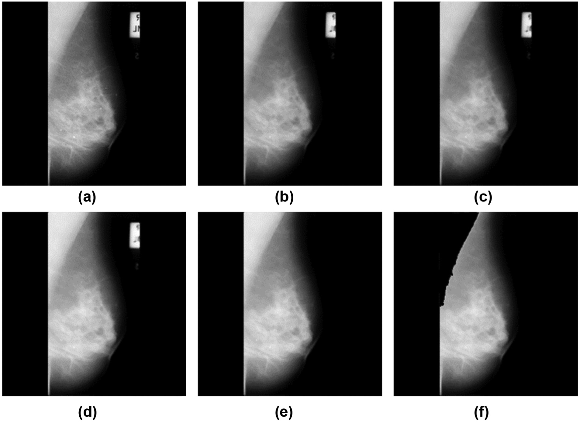
We picked up 200 samples from the dataset, 100 normal and 100 abnormal. The latter contains six types including calcification, architectural distortion, spiculated masses, circumscribed masses, ill-defined masses, and asymmetry (see Figure 2). Note that we treated all six types as abnormal, so our task is simplified as to detect abnormal breasts from normal ones.

Figure 2.

Illustration of six abnormal types: (a) circumscribed mass, (b) asymmetry, (c) architectural distortion, (d) calcification, (e) ill-defined masses, and (f) spiculated masses.

Methodology

Region-of-interest segmentation

In this step, we extracted the region of interest (ROI)^23–25 to avoid useless processing resources and data storage. The preprocessing is a five-step procedure as shown in Figure 3.

Figure 3.

Diagram of preprocessing.

In the first step, median filter (MF) is a nonlinear additive noise-reduction approach.²⁶ It can augment the performance of following processing. MF runs through the image pixel-by-pixel and replaces each pixel with the median of pixels within its approximated window. Usually, we force the window to contain an odd number of pixels, so the median operation is easy to implement. In this study, a 3 × 3 window was selected.

Next, homomorphic filtering (HF) was used to remove multiplicative noises. The diagram of HF is depicted in Figure 4.

Figure 4.

Diagram of HF.

Here, f and g represent the original and denoised image, respectively. DFT and IDFT means discrete Fourier transform and its inverse transform. The filter function H is defined as

H (u, v) = (a_{H} - a_{L}) [1 - \exp (- c \frac{D^{2} (u, v)}{D_{0}^{2}})] + a_{L}

(1)

where D₀ represents a specified distance; D(u, v) represents the distance from the point (u, v) to the origin; c is a constant to control the slope sharpness of the filter function; and a_L and a_H are defined as 0.5 and 2, respectively. Both “ln” and “exp” are logarithmic and exponential functions. Illumination and reflectance are combined in a multiplicative way,²⁷ the components are turned to be addictive by the logarithmic operation,²⁸ so they are separable in frequency domain.

Third, image enhancement is performed to give a better subjective view.²⁹ The image enhancement in spatial domain is the simplest method. Currently, there are three types of transform functions as linear, logarithmic, and power law. In this work, the logarithmic enhancement was used to expand the narrow range of low-level grayscale regions and shrinks the wide range of high-level grayscale regions.

Fourth, the background removal procedure removes the unwanted background contents, on the basis of the region-growing method, which relies on the hypothesis that neighboring pixels within a particular region entail similar gray values.³⁰ Region-growing method selects initial seed points and compares the seed points with their neighboring pixels. When a similarity criterion is met, then the neighboring pixels are assigned to the cluster that contains the seed points.³¹ The above process is iterated until all pixels in the image are segmented into clusters.

Finally, we need to remove the pectoral muscle area, which is usually denser than the normal breast tissue. This is done by applying a thresholding method, whose values were obtained by experience. After this step, the pectoral muscle was isolated and merely the ROI object remains within the mammogram image.

FRFT

In 2D situation, Fourier transform (FT) decomposes an image into frequency domain, and FT coefficients played an important role in many academic domains.³² A novel variant of FT, namely, FRFT was proven to have better performance than FT.³³

Suppose function x(t) is in the time domain (can be easily extended to 2D situation) and its α-angle FRFT spectrum X_α(f) is in the time–frequency domain, we have

X_{α} (f) = \int_{- \infty}^{\infty} S_{α} (t, f) x (t) d t

(2)

where S denotes the transform kernel with the form of

\begin{matrix} S_{α} (t, f) = \sqrt{1 - i \cot α} \\ \times \exp (i π (t^{2} \cot α - 2 ft \csc α + f^{2} \cot α)) \end{matrix}

(3)

where i is the imaginary unit. As α approaches a multiple of π, the operators csc and cot diverge. Taking the limit leads to the following clearer expression

S_{α} (t, f) = {\begin{matrix} \exp (i π (t^{2} \cot α - 2 ut \csc α + u^{2} \cot α)) \sqrt{1 - i \cot α} & α \neq m π \\ δ (t + f) & α = (2 m + 1) π \\ δ (t - f) & α = 2 m π \end{matrix}

(4)

where m is arbitrary integer and δ the Dirac delta function. Angular frequency ω can be used to replace time–frequency f so that

X_{α} (ω) = \int_{- \infty}^{\infty} S_{α} (t, ω) x (t) d t

(5)

here

\begin{matrix} S_{α} (t, ω) = \\ \sqrt{\frac{1 - i \cot α}{2 π}} \exp (i (\frac{t^{2} + ω^{2}}{2}) \cot α - t ω \csc α) \end{matrix}

(6)

For mammogram images, 2D-FRFT was implemented with two angles (α_x and α_y) involved. As α_x = α_y = 1, the FRFT turns to a standard FT. As α_x = α_y = 0, the FRFT turns to an identity operator. The 2D-FRFT can be performed by applying one one-dimensional (1D)-FRFT along rows and followed by applying another 1D-FRFT along columns or vice versa.³⁴

Weighted-type fractional Fourier transform and feature reduction

Weighted-type fractional Fourier transform (WFRFT) is the simplest calculation method of FRFT. It sticks to the rotation property of standard FRFT and meanwhile can be performed by fast algorithms. Mathematically, WFRFT replaced the continuous variables t with the discrete version n and replaced f with k. It defined by following form^35–37

F_{α} = \sum_{m = 0}^{3} a_{m} (α) F_{m}

(7)

a_{i} (α) = \frac{1}{4} \sum_{k = 1}^{4} \exp [i (α - m \frac{π}{2}) k]

(8)

From formula (7) we see that WFRFT is the linear combination of identity matrix, time inverse matrix, DFT matrix, and IDFT matrix. Nevertheless, the results of WFRFT are not strictly equal to those of FRFT,³⁸ that is, there will be slight changes for WFRFT results.

The WFRFT transforms the image to the fractional Fourier domain, and the obtained fractional Fourier spectrums contain too many features, which complicate the classification and increase computational burden. The PCA is able to reduce the data dimensionality in an efficient way. It uses a preset orthogonal transformation, so as to transform time–frequency coefficients X_α into new variables linearly uncorrelated. Those variables are named as principal components (PC).^39,40

Classification and cross validation

The reduced features were submitted to (1) SVM and (2) k-NN methods. SVM is the most popular classifier for small-size data. It is based on the principle of minimizing structural risk. The advantage of SVM is that it performs well on the test data, that is, its generalization ability is excellent.^41–43

k-NN is a simple yet robust nonlinear classifier.⁴⁴ It finds the k closest neighbors to the query sample and predicts it as the majority vote of classes of the k neighbors. The k-NN belongs to the instance-based learning, in which the functions are approximated locally and the training is deferred till classification.⁴⁵

The 10-fold stratified cross validation (SCV) was utilized to obtain out-of-sample error. The whole dataset was divided at random into 10 folds, with nearly the same distributions. Each time, nine folds are used for training and the rest for test. This procedure was repeated 10 times in the way that each fold was used as the test set. The classification performance was obtained by combination of all 10 results on the test set.

Above 10-fold SCV ran 50 times in order to eliminate the influence of randomness. The final performances based on a 50 × 10-fold SCV were yielded by calculating the average and standard deviation of the results of 50 runs. Three common measures were used as sensitivity, specificity, and accuracy.

Implementation

The implementation of this CAD system contains two phases. Phase I (offline learning) is to train the classifier and Phase II (online prediction) is to predict the result of query mammograms. Table 1 gives its pseudocode. Note that PCA in online prediction used the coefficient matrix generated by the PCA in offline learning.^46–48

Table 1.

Pseudocode of the proposed system.

Phase I: offline learning
Preprocessing	Users carried out preprocessing on all mammogram images. For a given image, users removed additive and multiplicative noises, enhanced the image, and removed background and pectoral muscle
Feature extraction	For a given mammogram, 16 time–frequency spectrum images were obtained by 16 different WFRFT operations with different combinations of α_x and α_y ([0.7 0.8 0.9 1.0] × [0.7 0.8 0.9 1.0])
Feature reduction	The 16 spectrum images were aligned into a vector as one observation and then PCA was performed over 200 mammograms. The threshold was to cover 95% variances
Training	The set of selected PCs together with the labels were submitted to train the classifiers (SVM and k-NN)
Evaluation	Report the performance based on a 50 × 10-fold SCV
Phase II: online prediction
Preprocessing	Users presented the query mammogram and performed the same preprocessing to segment the region of interest
Feature extraction	The 16 WFRFT spectrum images with the same pre-defined α_x and α_y were obtained
Feature reduction	The 16 WFRFT spectrum images were aligned and multiplied with PC coefficients, and the reduced features were yielded
Prediction	The reduced features were fed into the trained classifier, predicting the query mammogram as abnormal or normal

WFRFT: weighted-type fractional Fourier transform; PCA: principal component analysis; PC: principal component; SVM: support vector machine; k-NN: k-nearest neighbors; SCV: stratified cross validation.

Results and discussion

The algorithm was developed by ourselves based on 64-bit MATLAB 2015a (The Mathworks^©). Statistics toolbox was used to accelerate the program developing. The simulation experiments were implemented under Windows 7 operating system, on the platform of P4 IBM with 3.2-GHz processor and 8-GB RAM.

Preprocessing result

Figure 5 shows the result of each procedure during the preprocessing. Figure 5(a) shows an original image of a normal breast with dense glandular background. Figure 5(b) and (c) offers the noise-reduction results of additive noises and multiplicative noises. Here, we can observe the noises are nearly removed. Figure 5(d) provides the logarithmic contrast enhancement, by which the tissues in the mammogram are easily perceivable. Figure 5(e) and (f) takes away the background and pectoral muscle, respectively. In all, the ROI area was perfectly segmented.

Figure 5.

Each step of preprocessing: (a) original image, (b) additive noise reduction, (c) multiplicative noise reduction, (d) image enhancement, (e) background removal, and (f) pectoral muscle removal.

WFRFT of 1D simulation data

Figure 6 shows the time–frequency spectrum of a triangular signal tri(t). To show clearly how α affects the spectrum, α is assigned with 11 values from 0 to 1 with increase of 0.1. Remember that for a standard FT, the frequency spectrum turns the triangular signal to a 2-power of sinc function as sinc²(f).

Figure 6.

Time–frequency spectrums of tri(t): (a) 0, (b) 0.1, (c) 0.2, (d) 0.3, (e) 0.4, (f) 0.5, (g) 0.6, (h) 0.7, (i) 0.8, (j) 0.9, and (k) 1.0. Here, α is in the range of [0, 1]. The real components were plotted in black, while the imaginary components were plotted in blue.

The gradual change in Figure 6 shows the connection between time–frequency spectrum and the angle α. As α increases to 1, the time–frequency spectrum becomes standard frequency spectrum. As α decreases to 0, the time–frequency spectrum turns to original signal. Therefore, for the mammogram, we set both α_x and α_y vary from 0.7 to 1 with equal increase of 0.1. We did not consider the range in [0, 0.6] since FRFT with angles close to 0 will yield to original signal.

WFRFT of mammogram image

Figure 7 shows the different WFRFT spectrum images of a normal breast. Following the facts found in section “WFRFT of 1D simulation data,” we set the two angles α_x and α_y vary from 0.7 to 1 with equal increase of 0.1, respectively. Compared to standard FT that only transforms the mammogram image to one frequency spectrum, our defined WFRFT provides 16 spectrum images. Therefore, the WFRFT can provide more information than FT.

Figure 7.

Time–frequency spectrums of a normal breast. All images were log-enhanced and pseudocolor was added for clear vision.

Classifier comparison

The 16 spectrum images obtained by WFRFT were reduced by PCA and then the reduced features were fed into both SVM and k-NN. We compared “WFRFT+PCA+SVM” with “WFRFT+PCA+k-NN.” Here, SVM did not use any kernel. The optimal k in k-NN was obtained by grid searching, namely, from the range of [1, 9] with increment of 2. Finally, we found the k-NN achieved the largest accuracy when k was equal to 3. The results are listed in Table 2.

Table 2.

Classifier comparison.

Proposed method	Sensitivity	Specificity	Accuracy
WFRFT+PCA+SVM	92.22 ± 4.16	92.10 ± 2.75	92.16 ± 3.60
WFRFT+PCA+k-NN	91.18 ± 3.41	91.56 ± 3.28	91.37 ± 3.29

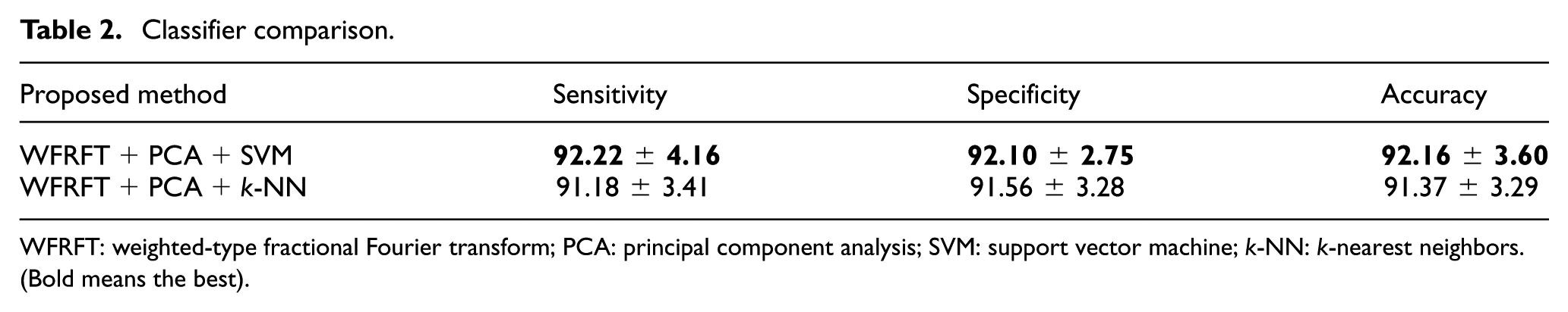
WFRFT: weighted-type fractional Fourier transform; PCA: principal component analysis; SVM: support vector machine; k-NN: k-nearest neighbors. (Bold means the best).

The comparison results in Table 3 show that the proposed “WFRFT+PCA+SVM” achieved sensitivity of 92.22% ± 4.16%, specificity of 92.10% ± 2.75%, and accuracy of 92.16% ± 3.60%. The proposed “WFRFT+PCA+k-NN” achieved sensitivity of 91.18% ± 3.41%, specificity of 91.56% ± 3.28%, and accuracy of 91.37% ± 3.29%. Hence, it is clear that using SVM obtained larger sensitivity, specificity, and accuracy than using k-NN. We can conclude that SVM is superior to k-NN in the diagnosis of abnormal breasts.

Table 3.

Classification comparison.

Authors	Methods	Sensitivity	Specificity	Accuracy
Milosevic et al.⁶	GLCM+SVM	20.4	87.2	62.0
Milosevic et al.⁶	GLCM+k-NN	38.9	73.8	60.7
Milosevic et al.⁶	GLCM+NBC	46.9	60.4	55.3
Yang et al.¹²	MIP+TPS	91.9 ± 2.3	70.0 ± 4.7	84.8 ± 3.1
Gorgel et al.¹⁹	SWT+SVM	93.3	88.6	90.1
Our method	WFRFT+PCA+SVM	92.22 ± 4.16	92.10 ± 2.75	92.16 ± 3.60

GLCM: gray-level co-occurrence matrix; NBC: naive Bayes classifier; MIP: maximum intensity projection; TPS: thin-plate spline; SWT: spherical wavelet transform; WFRFT: weighted-type fractional Fourier transform; PCA: principal component analysis; SVM: support vector machine; k-NN: k-nearest neighbors.

Comparison with state-of-the-art methods

We compared the better one of the two proposed methods, that is, the “WFRFT+PCA+SVM” with five state-of-the-art methods. The comparison results are shown in Table 3.

Data in Table 3 show that the “GLCM+SVM” approach obtained accuracy of 62.0%, “GLCM+k-NN” of 60.7%, “GLCM+NBC” of 55.3%, “MIP+TPS” of 84.8% ± 3.1%, and “SWT+SVM” of 90.1%. Our method obtains the largest accuracy of 92.16% ± 3.60%. Hence, this shows our method performs better than five state-of-the-art approaches. Another finding is WFRFT+PCA can extract more distinguishing features than GLCM, since the accuracy of “WFRFT+PCA+SVM” is larger than that of “GLCM+SVM.” This validates the superiority of WFRFT to GLCM.

Time analysis

Finally, we gave the time analysis of our WFRFT+PCA+SVM method over two stages: the offline learning (Phase I) and online prediction (Phase II). The results are shown in Table 4.

Table 4.

Time analysis (unit: second).

Phase I	Time
WFRFT	7914.33
PCA	0.48
SVM	0.69
Phase II	Time
WFRFT	38.15
PC score	0.02
SVM	0.01

WFRFT: weighted-type fractional Fourier transform; PCA: principal component analysis; SVM: support vector machine; PC: principal component.

The time analysis in Table 4 shows that Phase I costs about 7914.33+0.48+0.69 = 7915.5 s and Phase II costs about 38.15+0.02+0.01 = 38.18 s. Note that Phase I was performed over 200 mammogram images and Phase II was over one query image. A shortcoming of our approach is that the WFRFT process costs too much time (about 38.15 s per image). The reason is because the mammogram image is too large (1024 × 1024).

In the future, we will try to down-sample the mammogram images and test whether the classification performance will decrease. Besides, fast FRFT implementation methods will be included.^49,50

Conclusion and future research

We proposed a new approach for CAD of abnormal breast in mammogram images using the combination of three components: WFRFT, PCA, and SVM. The results show that our method yields better performance than five existing methods. Our contributions are as follows: (1) we apply WFRFT in abnormal breast detection and demonstrated WFRFT is effective and (2) the “WFRFT+PCA+SVM” is superior to state-of-the-art methods with regard to accuracy, sensitivity, and specificity.

In the future, thermograms will be considered. Besides, advanced classification methods (shared-weight neural network⁵¹ and deep learning⁵²) shall be included. The combination between WFRFT and entropy will also be considered as the fractional Fourier entropy. Another important thing is to apply our method to other diseases such as Alzheimer’s disease.

Footnotes

Academic Editor: António Mendes Lopes

Declaration of conflicting interests

The author(s) declared no potential conflicts of interest with respect to the research, authorship, and/or publication of this article.

Funding

The author(s) disclosed receipt of the following financial support for the research, authorship, and/or publication of this article: This paper was supported by NSFC (51407095 and 61503188), Natural Science Foundation of Jiangsu Province (BK20150983 and BK20150982), Jiangsu Key Laboratory of 3D Printing Equipment and Manufacturing (BM2013006), Key Supporting Science and Technology Program (Industry) of Jiangsu Province (BE2012201, BE2013012-2, and BE2014009-3), Program of Natural Science Research of Jiangsu Higher Education Institutions (15KJB470010, 13KJB460011, 14KJB480004, and 14KJB520021), Special Funds for Scientific and Technological Achievement Transformation Project in Jiangsu Province (BA2013058), Nanjing Normal University Research Foundation for Talented Scholars (2013119XGQ0061 and 2014119XGQ0080), and Open Fund of Guangxi Key Laboratory of Manufacturing System & Advanced Manufacturing Technology (15-140-30-008K).

References

Teh

Tan

G-H

Taib

. Opportunistic mammography screening provides effective detection rates in a limited resource healthcare system. BMC Cancer 2015; 15: 6.

Henderson

O’Meara

Braithwaite

. Performance of digital screening mammography among older women in the United States. Cancer 2015; 121: 1379–1386.

Hartman

Drotman

Arleo

EK.

Annual screening mammography for breast cancer in women 75 years old or older: to screen or not to screen. Am J Roentgenol 2015; 204: 1132–1136.

Zhang

Wang

Phillips

. Three-dimensional eigenbrain for the detection of subjects and brain regions related with Alzheimer’s disease. J Alzheimers Dis 2016; 50: 1–18.

Wang

Zhang

Liu

. Detection of Alzheimer’s disease by three-dimensional displacement field estimation in structural magnetic resonance imaging. J Alzheimers Dis 2016; 50: 233–248.

Milosevic

Jankovic

Peulic

Comparative analysis of breast cancer detection in mammograms and thermograms. Biomed Tech 2015; 60: 49–56.

Azar

El-Said

. Performance analysis of support vector machines classifiers in breast cancer mammography recognition. Neural Comput Appl 2014; 24: 1163–1177.

Iseri

Computer aided detection of microcalcification clusters in mammogram images with machine learning approach. Optoelectron Adv Mat 2014; 8: 689–695.

Han

Chen

. Mass segmentation in mammogram based on SPCNN and improved vector-CV. Acta Phys Sin 2014; 63: 11.

10.

Singh

Jain

Singh

Mammogram mass classification using support vector machine with texture, shape features and hierarchical centroid method. J Med Imaging Health Inform 2014; 4: 687–696.

11.

Perez

Guevara López

Silva

. Improving the Mann-Whitney statistical test for feature selection: an approach in breast cancer diagnosis on mammography. Artif Intell Med 2015; 63: 19–31.

12.

Yang

Liao

. Identification of breast cancer using integrated information from MRI and mammography. Plos ONE 2015; 10: 11.

13.

Yakoumakis

Tzamicha

Dimitriadis

. Dual-energy contrast-enhanced digital mammography: patient radiation dose estimation using a Monte Carlo code. Radiat Prot Dosimetry 2015; 165: 369–372.

14.

Zheng

Keller

Ray

. Parenchymal texture analysis in digital mammography: a fully automated pipeline for breast cancer risk assessment. Med Phys 2015; 42: 4149–4160.

15.

Anitha

Peter

JD.

Mammogram segmentation using maximal cell strength updation in cellular automata. Med Biol Eng Comput 2015; 53: 737–749.

16.

Peng

Chou

Pan

. FDG-PET/CT detection of very early breast cancer in women with breast microcalcification lesions found in mammography screening. J Med Imaging Radiat Oncol 2015; 59: 445–452.

17.

Molloi

Ding

Feig

Breast density evaluation using spectral mammography, radiologist reader assessment, and segmentation techniques: a retrospective study based on left and right breast comparison. Acad Radiol 2015; 22: 1052–1059.

18.

Nithya

Santhi

Computer aided diagnosis system for mammogram analysis: a survey. J Med Imaging Health Inform 2015; 5: 653–674.

19.

Gorgel

Sertbas

Ucan

ON.

Computer-aided classification of breast masses in mammogram images based on spherical wavelet transform and support vector machines. Expert Systems 2015; 32: 155–164.

20.

Seok

Bae

Target classification using features based on fractional Fourier transform. IEICE T Inf Syst 2014; E97D: 2518–2521.

21.

Bhaduri

Tay

Quan

. Motion detection using extended fractional Fourier transform and digital speckle photography. Opt Express 2010; 18: 11396–11405.

22.

Ajmera

Holambe

RS.

Fractional Fourier transform based features for speaker recognition using support vector machine. Comput Electr Eng 2013; 39: 550–557.

23.

Vitrani

Marx

Iordache

. Robot guidance of an ultrasound probe toward a 3D region of interest detected through X-ray mammography. Int J Comput Assist Radiol Surg 2015; 10: 1893–1903.

24.

Shang

Guo

Liu

. Finding regions of interest using location based social media. Neurocomputing 2016; 173: 18–123.

25.

Chen

Zhang

Yang

. Curve-like structure extraction using minimal path propagation with back-tracing. IEEE T Image Process 2016; 25: 988–1003.

26.

Cadenas

Megson

Sherratt

RS.

Median filter architecture by accumulative parallel counters. IEEE T Circuits: II 2015; 62: 661–665.

27.

Sharma

Bhagat

OL.

Respiratory rate extraction from single-lead ECG using homomorphic filtering. Comput Biol Med 2015; 59: 80–86.

28.

Shahamat

Pouyan

AA.

Face recognition under large illumination variations using homomorphic filtering in spatial domain. J Vis Commun Image R 2014; 25: 970–977.

29.

Almuntashri

Agaian

Human visual system-based edge detection using image contrast enhancement and logarithmic ratio. In: Mobile multimedia/image processing, security, and applications, vol. 7708, Orlando, FL, 2 April 2010, p.11. Bellingham WA: SPIE.

30.

Mallikarjunaswamy

Holi

Raman

Knee joint menisci segmentation, visualization and quantification using seeded region growing algorithm. J Med Imaging Health Inform 2015; 5: 552–560.

31.

Truong-Hong

Laefer

. Octree-based region growing for point cloud segmentation. ISPRS J Photogramm 2015; 104: 88–100.

32.

Pajares

Sensors and technologies in Spain: state-of-the-art. Sensors 2014; 14: 15282–15303.

33.

Zhang

Y-D

Chen

Wang

S-H

. Magnetic resonance brain image classification based on weighted-type fractional Fourier transform and nonparallel support vector machine. Int J Imag Syst Tech 2015; 25: 317–327.

34.

Cagatay

Datcu

FrFT-based scene classification of phase-gradient InSAR images and effective baseline dependence. IEEE Geosci Remote S 2015; 12: 1131–1135.

35.

Shih

C-C.

Fractionalization of Fourier transform. Opt Commun 1995; 118: 495–498.

36.

Santhanam

McClellan

JH.

The discrete rotational Fourier transform. IEEE T Signal Process 1996; 44: 994–998.

37.

Wang

Zhang

Yang

. Pathological brain detection by a novel image feature—fractional Fourier entropy. Entropy 2015; 17: 7877.

38.

Ozaktas

Arikan

Kutay

. Digital computation of the fractional Fourier transform. IEEE T Signal Process 1996; 44: 2141–2150.

39.

Kuroda

Mori

Iizuka

. Acceleration of the alternating least squares algorithm for principal components analysis. Comput Stat Data An 2011; 55: 143–153.

40.

Zhang

Classification of fruits using computer vision and a multiclass support vector machine. Sensors 2012; 12: 12489–12505.

41.

Fernández

Ahmad

Abreu

. Large-scale recognition of high-affinity protease-inhibitor complexes using topological autocorrelation and support vector machines. Mol Simulat 2016; 42: 420–433.

42.

Dalei

Mohanty

KB.

Fault classification in SEIG system using Hilbert-Huang transform and least square support vector machine. Int J Elec Power 2016; 76: 11–22.

43.

Zhang

Wang

Phillips

. Detection of Alzheimer’s disease and mild cognitive impairment based on structural volumetric MR images using 3D-DWT and WTA-KSVM trained by PSOTVAC. Biomed Signal Proces 2015; 21: 58–73.

44.

Chavez

Graff

Navarro

. Near neighbor searching with K nearest references. Inform Syst 2015; 51: 43–61.

45.

Formoso

Fernández

Cacheda

. Distributed architecture for k-nearest neighbors recommender systems. World Wide Web 2015; 18: 997–1017.

46.

Zhang

Dong

Wang

. Preclinical diagnosis of magnetic resonance (MR) brain images via discrete wavelet packet transform with Tsallis entropy and generalized eigenvalue proximal support vector machine (GEPSVM). Entropy 2015; 17: 1795–1813.

47.

Hron

Menafoglioc

Templ

. Simplicial principal component analysis for density functions in Bayes spaces. Comput Stat Data An 2016; 94: 330–350.

48.

Shams-Nateri

Piri

Prediction of emission spectra of fluorescence materials using principal component analysis. Color Res Appl 2016; 41: 16–21.

49.

Kumari

Thanushkodi

A secure fast 2D—discrete fractional Fourier transform based medical image compression using hybrid encoding technique. In: 2013 international conference on current trends in engineering and technology (ICCTET), Coimbatore, India, 3 July 2013, pp.1–7. New York: IEEE.

50.

Campos

Rico-Melgoza

Chavez

A new formulation of the fast fractional Fourier transform. SIAM J Sci Comput 2012; 34: A1110–A1125.

51.

Wang

Chen

. Detection of dendritic spines using wavelet-based conditional symmetric analysis and regularized morphological shared-weight neural networks. Comput Math Method M 2015; 2015: 454076 (12 pp.).

52.

Hou

Eickholt

. Improving protein fold recognition by deep learning networks. Sci Reports 2015; 5: 17573 (11 pp.).

Computer-aided diagnosis of abnormal breasts in mammogram images by weighted-type fractional Fourier transform

Abstract

Keywords

Background

Materials

Methodology

Region-of-interest segmentation

FRFT

Weighted-type fractional Fourier transform and feature reduction

Classification and cross validation

Implementation

Results and discussion

Preprocessing result

WFRFT of 1D simulation data

WFRFT of mammogram image

Classifier comparison

Comparison with state-of-the-art methods

Time analysis

Conclusion and future research

Footnotes

Declaration of conflicting interests

Funding

References