Sage Journals: Discover world-class research

Abstract

Through the convergence analysis of the iterative learning control, it can be seen that the inverted model of the sensitivity can be used as the update law of iterative learning controller. However, due to the little knowledge in modeling uncertainty and in feedback controllers embedded in drivers with hard-to-obtain parameters, it is difficult to directly calculate the transfer function of the sensitivity. To solve this problem, this article presents sensitivity identification–based iterative learning controller for a high-acceleration positioning table actuated by the voice coil motors. In the sensitivity identification process, a frequency sweep signal was exerted to the closed-loop system as the equivalent disturbance, and the perturbation of the tracking error was gathered as output data. Then, the autoregressive model of the sensitivity was gained conveniently. Finally, the proposed sensitivity identification–based iterative learning controller was implemented in the experimental setup with the maximum acceleration of 5.3 g. The experimental results show that the tracking error of the X- and Y-axes decreased from 530 and 2480 µm to 6 and 18 µm, respectively, after the third iteration of the proposed iterative learning controller method, and the identified sensitivity can be easily designed in the iterative learning controller to greatly improve the tracking performance.

Keywords

Precise positioning table high acceleration iterative learning controller sensitivity identification

Introduction

Fast trajectory tracking motions with high acceleration and high operating speed are widely applied in the semiconductor industry, for example, in wire bonding and die mounting.¹ The product performance and production efficiency of such needs depend on their motion accuracy. Aside from the positioning accuracy, another important characteristic of precision positioning machines is high responsiveness, that is, high acceleration and high velocity.² Recently, many precision positioning tables driven by a linear motor (LM) are widely used to perform such motion tasks.³ However, the systems operated at high acceleration are still subjected to many uncertain factors. First, it is well known that the direct drive tables are very sensitive to external disturbance, unmodeled dynamics, and nonlinearity, so there is a high need for the robustness of the control system. Second, these systems usually adopt higher system gains to enlarge control bandwidth, reduce tracking errors, and improve the dynamic features;⁴ however, higher gains will destroy the system stability.⁵ Specifically speaking, these are great challenges for the high-precision motion controller design of these high-acceleration systems.

To investigate the method for trajectory tracking and good disturbance rejection ability in high-speed and high-precision system, scholars explore many kinds of advanced theories and methods. Adaptive control is useful in a system wherein the nonlinearity can be linearly parameterized, but in practical rapid dynamic situation, the adaptive control law is not a good option, and a small disturbance may cause instability.⁶ An alternative approach, such as robust control method, is proposed to combat the uncertainties of the parameters and the disturbances, including sliding mode variable structure control,^7,8 which is an effective approach for the system with unmodeled dynamics. Its main drawback is that it utilizes a discontinuous function, that is, a sign function, thus causing severe chattering across the sliding surface⁹ and correspondingly affecting the system’s control performance. To overcome full-scale disturbances, a disturbance observer¹⁰ has been widely used in engineering practice. Although the design of an observer is based on the mathematical modeling of low-frequency plant dynamics, it is hard to obtain the accurate system model especially in rapid dynamic response. Furthermore, all the works above can achieve high-precision and high-acceleration motion only by changing the parameters of controller through trial and error; but in industry application, the controller is usually embedded in the system, the user only has partial knowledge about the controller structure, and this situation results in difficulties in application to adjust control gains. An alternative approach to achieve high-acceleration motion and to overcome the limitation of the industry application is through the addition of feedforward compensator with existing feedback loop.

It is well known that iterative learning controller (ILC) is an optional scheme for achieving the positioning control with high precision and fast system response by means of repetitive learning. The problem of iteratively learning and controlling a system can be expressed as the iterative modification of the system input to minimize the tracking error.¹¹ ILC is essentially a feedforward control approach that fully utilizes the past control information.¹² It means that ILC can be designed as an add-on controller over an existing feedback loop. G Parmar et al.¹³ applied a P-type ILC controller in conjunction with linear feedback in a single-axis motion table, and during 20–30 times learning, the tracking error was reduced by second order of magnitude in high-speed, rapid dynamic motion. However, the convergence speed of P-type ILC controller is so slow such that the learning controller is hardly promoted and applied in industry scene. To further improve the convergence speed of ILC algorithm with closed loop, a model-based method for choosing an ILC controller is presented in Merry et al.¹⁴ and Owens et al.¹⁵ By deriving the convergence of ILC in closed loop, the inverted model of sensitivity as defined by the transfer function between the disturbance and tracking error in the feedback loop is a suitable choice for the ILC update law. It overcomes the limitations of slow convergence with P-type ILC, and the modeling uncertainty may be tolerated by a feedback controller. However, obtaining the transfer function of the sensitivity is the key problem in the model-based ILC design. A fatal disadvantage of this model-based ILC controller is that the transfer function of the sensitivity depends on the feedback controller structure and the controlled object plant. But due to the little knowledge of feedback controller in real industrial processes and many feedback controllers embedded in drivers, the detailed parameters of controlled object are hard to obtain. Therefore, it is very difficult to determine the transfer function of the sensitivity by direct calculation.

Aiming at a solution for the above-mentioned problems, this article proposes a sensitivity identification (SI) approach–based ILC. This method is completely independent of the knowledge of plant and feedback controller. On the basis of a feedforward compensation constructed by ILC, it overcomes the limitations of slow convergence with P-type ILC and acquires asymptotic tracking error convergence rapidly. Based on the definition of sensitivity, evidently, through adding a bounded excitation signal to the analog-to-digital converter (ADC) port as an outside equivalent disturbance input, the perturbation of tracking error can be brought into the closed-loop system. Then, the perturbation of the tracking error, which can characterize the robustness of the closed loop, is gained as the output of the sensitivity plant. Furthermore, the response of the tracking error and the excitation signal can be viewed as frequency sweep modeling (FSM) data, which characterize the plant of sensitivity. By this way, an autoregressive exogenous (ARX) model of the sensitivity is conveniently obtained according to appropriate FSM. After the sensitivity inversing operation, the ILC update law is successfully applied via SI. Finally, the SI-based ILC is implemented on a high-acceleration positioning table experimental setup in which the feedback control is embedded in the programmable multi-axes controller (PMAC) card. The experimental results show that the tracking error is reduced with a few iterations, and because the compensation is realized by feedforward control, the control accuracy can also be enhanced without changing the structure of feedback controller.

The remainder of this article is organized as follows: in section “Experimental setup of high-acceleration positioning table,” the experimental setup is discussed; a novel method to design an ILC controller via SI approach is presented in section “Controller design”; the results of the experiments are discussed in section “Experimental results”; and finally, the conclusions are given in section “Conclusion and discussion.”

Experimental setup of high-acceleration positioning table

The experimental platform is a decoupling X–Y motion table driven by a voice coil motor (VCM), which is shown in Figures 1 and 2. The VCM is a direct driving LM that can eliminate the influence of backlash between gear pair and gear transmission. In addition, it has the feature of no cogging effect, fast response, large thrust, and high-frequency response. The stage has the weight of 2.225 kg, and both axes travel at the range of 50 mm, and a decoupling mechanism was applied to reduce the motion inertia. The two axes were individually driven by two linear amplifiers TA330-E01 that can output pure analog quantity with a high-resolution ratio and avoid losses in the process of digital switching with distortion near zero. The selected detecting components are the precise raster produced by the company RENISHAW whose resolution is 0.1 µm. A PMAC clipper with superior performance was selected as the cybernetics core. In the control system, the commands from host PC were transmitted to PMAC via TCP/IP. The core of the PMAC is a digital signal processor, which is a special type of microprocessor optimized for fast and repeated mathematical operations of the type found commonly in motion control. In addition, the servo cycle of PMAC was set as 0.404 ms while ensuring control precision and eliminating the ripple. The output signal drives the VCM to perform the corresponding motions through the amplifier, and simultaneously, the raster detects the current location information and gives feedback to the control card, thus forming a closed-loop control.

Figure 1.

Structure of X–Y motion table.

Figure 2.

Structure of the experimental system.

The ILC controller was implemented in a host computer through calculating the update feedforward offline. The host computer sends the feedforward data of iterative computation into the registers of PMAC. During the next sample of tracking motion, the feedforward data, which are saved in registers, will compensate the error by modifying the offset digital-to-analog converter (DAC) port of PMAC. Through this way, the ILC controller was independent of the feedback controller and had no effects on the stability of the control system.

Controller design

In this section, the whole structure of the controller, as shown in Figure 3, includes a block diagram of a system Plant P with proportional–derivative (PD) feedback and ILC controllers. ILC reduces the repetitive part of the error e_k = y_d − y by updating the feedforward signal U_k_+ 1 by following the update law H, in which the H is determined by SI approach. The remaining part of the ILC controller is a low-pass filter Q, and a register (memory) is used to save the last feedforward signal U_k. The PD feedback controller improves the ability of restraining the parameter perturbation, stochastic distribution, and the robust performance of the controlled system. In the PD feedback controller, K_p, K_v, and S refer to the proportional gain, derivative gain, and differentiation element, respectively. In particular, y_d denotes the anticipated trajectory input, and y is the real output. The structure of the PD controller was selected by default setting on the Turbo PMAC, and the parameters of the controller were chosen to satisfy the bandwidth as well as the robust stability of the system.

Figure 3.

Block diagram of the controller based on ILC.

The ILC feedforward signal U_k_+ 1 was updated offline, that is, between successive iterations, while the error e_k was filtered by a learning filter H and was added to the feedforward U_k. The sum of filtered error and the last feedforward signal U_k was applied to obtain the feedforward signal for the next iteration U_k_+ 1 through filter Q. From the analysis above, it can be seen that the main point for developing ILC controller is the learning update law H and filter Q. In the rest of this section, the research will be focused on them. Therefore, in subsection “ILC,” the general method of an ILC update law is introduced, and the theoretical convergence condition is also deduced. Based on the deduced update law (sensitivity) in subsection “ILC,” the SI approach is proposed in subsection “Identification of the sensitivity,” and some key details are also pointed out.

ILC

This part will briefly introduce the method of ILC update law design and the definition of sensitivity. However, before discussing how to design the ILC learning update law, one should simplify the block diagram of the controller to general form as shown in Figure 4. Here, C denotes the feedback controller, which can be obtained by block diagram reduction.

Figure 4.

Block diagram with simplest feedback controller.

From the Figure 4, the transfer function from feedforward U_k to error can be derived, and that is defined as sensitivity function, which shows how sensitive tracking error is to outside disturbance

S_{p} = \frac{- e_{k}}{U_{k}} = \frac{P}{1 + CP}

(1)

One of the performance objectives of controller design is to keep the error as small as possible when the closed-loop system is affected by external signals. Thus, to be able to assess the relationship between the disturbance and the process output, the concepts of sensitivity are to be introduced. By analyzing the convergence of ILC in the following part, the reason why the inverted model of sensitivity as the learning update law was chosen is given.

The learning update of the feedforward signal equals

U_{k + 1} = U_{k} + H e_{k}

(2)

and the propagation of the error from iteration to iteration can be written as

e_{k + 1} = \frac{- P}{(1 + CP) U_{k + 1}} = \frac{- P}{(1 + CP) (U_{k} + H e_{k})} = e_{k} ((\frac{1 - P}{1 + CP}) H)

(3)

According to the fixed point principle, the necessary and sufficient condition for the error convergence is^16,17

‖ 1 - P (1 + CP) H ‖_{\infty} < 1

(4)

and the suitable choice for the learning update law H would be

H = S_{p}^{- 1} = {(\frac{P}{1 + CP})}^{- 1}

(5)

As the S_P of this system is a non-minimum phase system, the stability of the sensitive function in the inverse model is the premise for assuring the operation of the method. However, when the sensitive function of the inverse model includes the zero point on the unit circle or the zero point outside the unit circle, the direct inverse operation will produce the pole, which leads to instability. Therefore, zero phase error tracking control (ZPETC)¹⁸ is introduced to design the sensitive function inversion

S_{p}^{- 1} = \frac{A_{c} (z^{- 1}) B^{u} (z)}{z^{- d} B^{a} (z^{- 1}) {[B^{u} (1)]}^{2}}

(6)

The polynomials B^u include all the unstable zero points on and outside the unit circle. The polynomials B^a include all the stable zero points in the unit circle. The polynomials A_c include all the pole points in the original sensitive function.

As shown in Figure 4, the learning update of the feedforward command of ILC equals

u_{k + 1} = Q (u_{k} + e_{k} {(\frac{P}{1 + CP})}^{- 1})

(7)

Identification of the sensitivity

According to the analyses above, it can be found that the law of learning update, as shown in equation (7), is the key part of ILC design. It can also be noted that the learning update law depends on the feedback controller structure and the controlled object plant. Although the controlled object P in learning update law can be modeled by mathematical method or system identification, there are such obvious differences in acquiring the precise control structure C and its parameters. To directly obtain the sensitivity and avoid troubles in determining the parameters and the structure of controller, the definitions of sensitivity should be taken into consideration. As Figure 5 denotes, a frequency sweep signal is input as the equivalent disturbance to the closed-loop systems, which is generated by MATLAB function chirp. At the same time, one reference signal is set to maintain zero and get the tracking error, which is caused by the equivalent disturbance signal. Furthermore, the response of the tracking error and the excitation signal can be viewed as FSM data. In this way, the ARX model of the sensitivity is obtained according to the appropriate excitation signal of identification.

Figure 5.

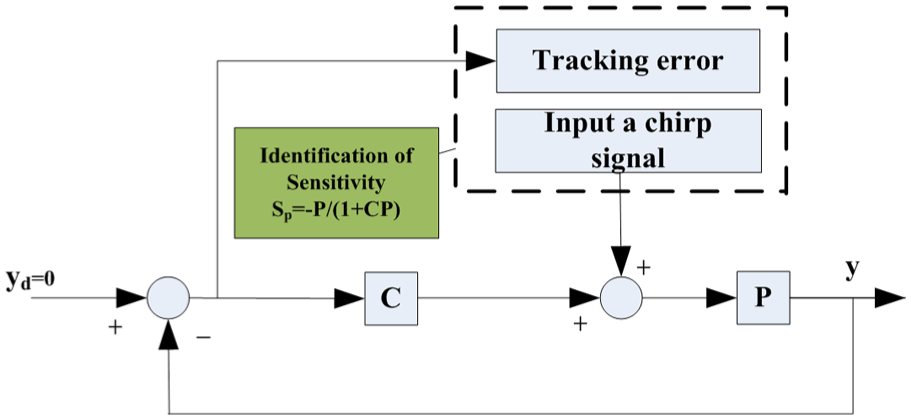
Identification of the sensitivity.

It is significant to analyze the appropriate frequency range and the gain of the FSM signal. To excite the system in full band, 200 Hz bandwidth of sweep signal should be selected. The maximum scan frequency is determined by the maximum acceleration of the system. In order to prevent the effect of friction nonlinearity, the amplitude of the signal should be large enough. For example, considering the Y-axis, the input sweep magnitude frequency varies from 2 to 200 Hz whose magnitude is 500 mV. Finally, the identification signal is put into the ADC port, holding the reference input at zero at the same time. Then, the response of tracking error can be gathered as shown in Figure 6.

Figure 6.

Data of frequency sweep modeling: (a) FSM data of X-axis and (b) FSM data of Y-axis.

After the experiment in FSM, the next goal of identification is to get the plant of sensitivity. Generally, the modeling for sensitivity is quite complex, and it is difficult to know the model structure, especially for the case wherein the mechanical system has nonlinear parts or unknown structures. When the controller’s internal structure is unknown, the ARX model, a kind of input–output polynomial model, is completely suitable for the sensitivity modeling. A more compact way to write the ARX model equation is

A (q) y (t) = B (q) u (t - n_{k}) + e_{m} (t)

(8)

where q is the delay operator, and $e_{m} (t)$ is the modeling error

A (q) = 1 + a_{1} q^{- 1} + \dots + a_{n_{a}} q^{- n_{a}}

(9)

B (q) = b_{1} + b_{2} q^{- 1} + \dots + a_{n_{b}} q^{- n_{b} + 1}

(10)

where n_a means order of the polynomial A(q), and n_b means order of the polynomial B(q) in equation (10). a and b denote the corresponding coefficients of numerator and denominator. The specific procedures are as follows:

Combine the input, output, and the sample time into a MATLAB identification format “iddata.”;

Confirm the number of identifying parameters and order of plant;

Deal this “iddata” with an arx(iddata, [n_a n_b, q]) function of MATLAB Identification Toolbox to get discrete-time ARX structure polynomial model of sensitivity with estimated parameters of model using the least-squares method and specified orders.

As this method belongs to black-box modeling, the key lies should confirm the number of identifying parameters and the order of plant. By testing different combination modes of identifying orders in modeling sensitivity, the results prove that the influences of various order of identifying parameters in modeling are clearly different, the effects of different identifying parameters in sensitivity modeling are shown in Table 1 and Figure 7. Table 1 shows the Y-axis’ identifying parameters. (4, 3) and (4, 2) are slightly worse. (5, 4) and (5, 3) have almost identical mean squared error (MSE) and final prediction error (FPE) when both Y-axis and X-axis were considered. (5, 4) can better describe the flexibility of X-axis. In order to solve unified model, (5, 4) was selected.

Table 1.

Effects of different identifying parameters on sensitivity modeling.

(n_b/n_a)	(2, 1)	(3, 1)	(3, 2)	(4, 2)	(4, 3)	(5, 3)	(5, 4)	(6, 4)	(6, 5)
FPE	2.277	0.8709	0.8932	0.5523	0.5498	0.515	0.5129	0.5041	0.4965
MSE	2.274	0.8691	0.8919	0.5513	0.5487	0.5138	0.5115	0.5026	0.4949
Fit (%)	99.49	99.68	99.68	99.75	99.75	99.76	99.76	99.76	99.76

FPE: final prediction error; MSE: mean squared error.

Figure 7.

Different orders of identifying parameters affect the modeling accuracy.

After the experiment in FSM, the sensitivity function can be obtained through arx() function according to the number of identifying parameters conformed above. Then, the ARX model of the sensitivity can be expressed in discrete type

S_{p - x} = \frac{- 0.27792 z (z + 2) (z - 1.7101) (z - 0.6685)}{(z - 0.9046) (z^{2} - 1.798 z + 0.8911) (z^{2} + 0.909 z + 0.3771)}

(11)

S_{p - y} = \frac{- 0.095039 z (z - 2.348) (z + 0.8669) (z - 0.2666)}{(z - 0.8693) (z^{2} - 1.762 z + 0.8361) (z^{2} + 0.824 z + 0.2647)}

(12)

The bode diagram of the sensitivity function is displayed in Figure 8. Because when the mechanical rigidity of X-axis is lower than Y-axis, there is a more obvious resonance point in the bode diagram.

Figure 8.

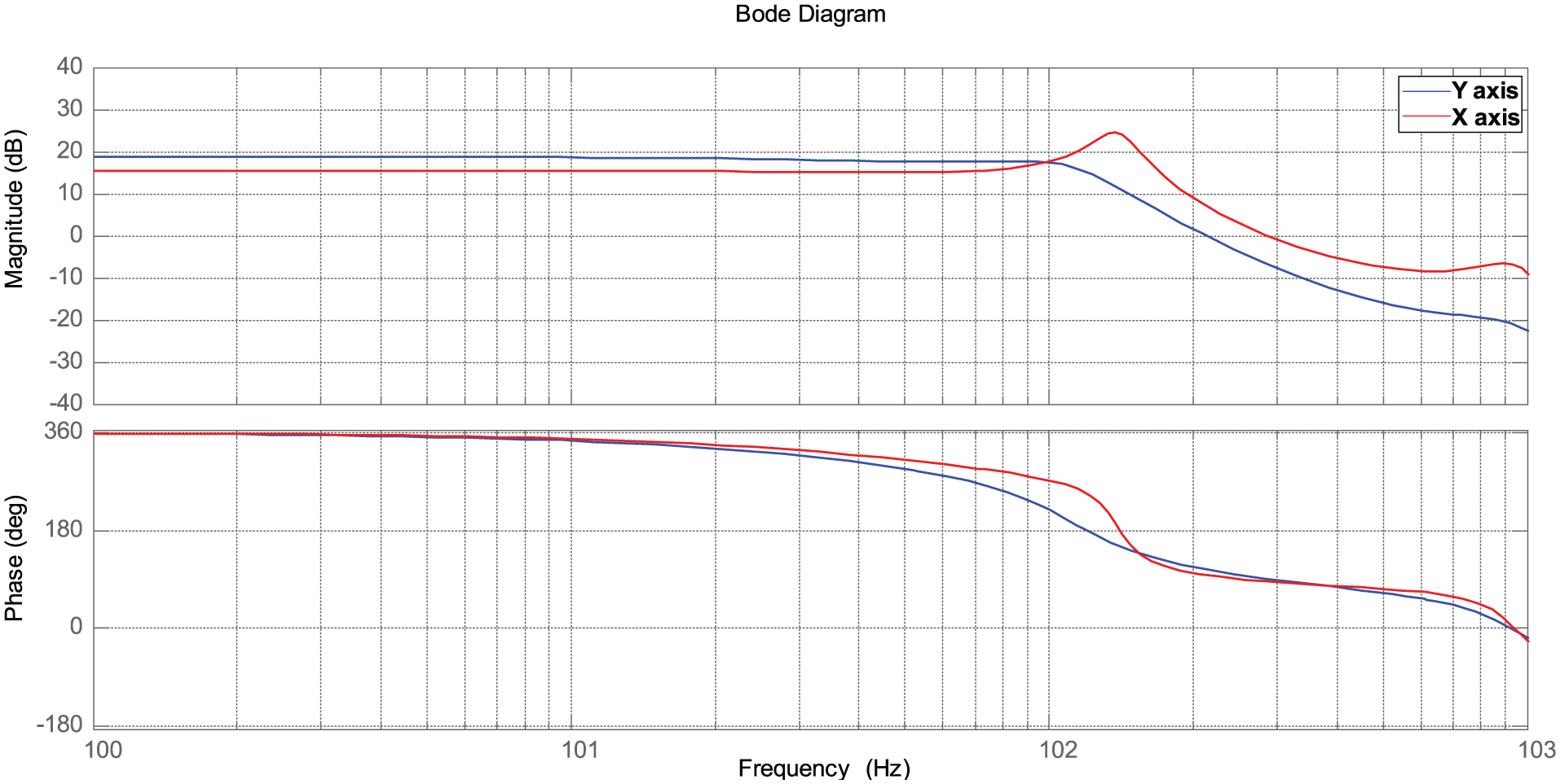
Bode plot of the sensitivity.

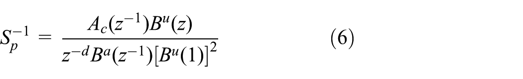
Then, the identified sensitivity described above was applied to the update law of the ILC controller (equation (7)). Therefore, the inverse of the sensitivity should be obtained by substituting equations (11) and (12) in equation (6). It can be seen that this sensitive function includes some zero points that are out of unit circle, and the approximate stable inverse model can be obtained

S_{p - x}^{- 1} = \frac{3.421 z^{6} - 6.418 z^{5} + z^{4} + 3.268 z^{3} - 0.1667 z^{2} - 1.5701 z + 0.1269}{1.261 z^{4} + 0.8431 z^{3}}

(13)

S_{p - y}^{- 1} = \frac{2.348 z^{6} - 5.242 z^{5} + 2.897 z^{4} + 0.7737 z^{3} - 0.4618 z^{2} - 0.4796 z + 0.1924}{0.1727 z^{4} + 0.1036 z^{3} - 0.0399 z^{2}}

(14)

Sensitivity $S_{p}$ is usually regarded as signaling system that has low-pass attribute. Thus, most of the high-frequency noise will be introduced when the controller choose inverted sensitivity. In particular, a low-pass filter Q should be designed after $S_{p}^{- 1}$ to be sure that the feedforward compensation channel is stable. Meanwhile, a fourth-order Butterworth filter with a bandwidth of 100 Hz was used to insure the convergence and good tracking performance. The servo cycle of PMAC was set as 0.404 ms while ensuring control precision and eliminating the ripple; then, the discrete transfer function Q could be written as

Q (z) = \frac{0.0004166 z^{4} + 0.001666 z^{3} + 0.002500 z^{2} + 0.001666 z + 0.0004166}{z^{4} - 3.181 z^{3} + 3.861 z^{2} - 2.112 z + 0.4383}

(15)

Experimental results

In this section, the proposed ILC controller with SI method was implemented on the high-acceleration positioning table as shown in Figure 3. According to the rise time and the overshoot of the step response, the PD controller parameters were chosen as K_p = 1100 and K_d = 550. The motion profile was set as a point-to-point profile with five-order displacement curve for least vibrations at the motion end, and the expression is written as

{\begin{matrix} A [6 {(\frac{t}{T_{r}})}^{5} - 15 {(\frac{t}{T_{r}})}^{4} + 10 {(\frac{t}{T_{r}})}^{3}], 0 ⩽ t ⩽ T_{r} \\ A, t > T_{r} \end{matrix}

(16)

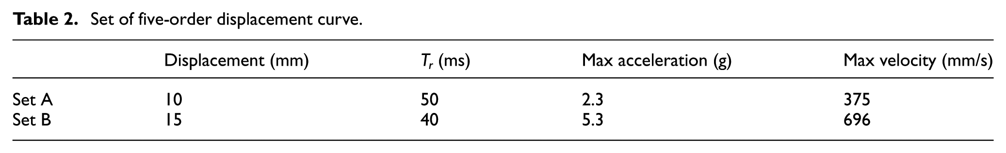
where A denotes the max displacement, and T_r denotes the rise time of the curve. It can be inferred that T_r and A of the five-order displacement curve exert the effect of the acceleration and velocity of the curve. A number of experimental profiles were used to verify the tracking performance of high acceleration. Hence, the displacements in the experiment included different maximum accelerations, and Table 2 shows the different sets of curve parameters.

Table 2.

Set of five-order displacement curve.

	Displacement (mm)	T_r (ms)	Max acceleration (g)	Max velocity (mm/s)
Set A	10	50	2.3	375
Set B	15	40	5.3	696

In the first situation, Set A–desired trajectory was implemented in the X–Y motion table, the tracking performance was obtained after several iterations, and the results are shown in Figure 9. The detailed performance is also summarized in Table 4. It can be seen that the ILC with SI method markedly reduced the max tracking error after three iterations of learning, the maximum tracking errors of X- and Y-axes were reduced from 1200 and 180 µm to 6 and 4.5 µm, respectively; and correspondingly, the positioning times were shortened from 66 and 60 ms to 40 and 50 ms, respectively.

Figure 9.

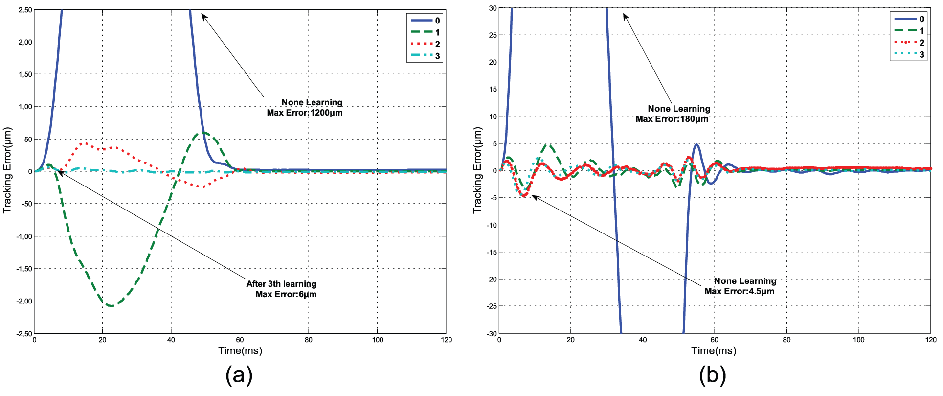
Tracking errors of profile Set A (2.3 g): legend shows number of learning iterations (0 = no learning): (a) tracking error of X-axis and (b) tracking error of Y-axis.

In the condition of high-acceleration situation, profile Set B was introduced to the X–Y motion table. The tracking performances for both X- and Y-axes are shown in Figure 10. In Tables 3 and 4, it can be seen that the maximum tracking errors of X-axis was still reduced from 1200 and 2480 µm to 6 and 18 µm, respectively, after three times learning, and the detailed performance indices are also summarized in Table 4. The tracking performance of X-axis is slightly inferior to that of Y-axis without ILC. The main reason is that the decoupling mechanism of X-axis weakens the rigidity of the system and causes lag, so there is zero overshoot without ILC. After iterative learning control, the performance of the X-axis is close to the Y-axis, and there is some overshot using ILC. It means that the iterative learning can compensate the inherent defects of the mechanical system and improve the system performance. It can be found that the ILC with SI method can shorten the time of location and improve the precision even in high acceleration through several iterations. That is to say, compared to Set A (2.3 g) profile, the ILC with SI method can also play a positive role in higher acceleration profile (5.3 g).

Figure 10.

Tracking errors of profile Set B (5.3 g): legend shows number of learning iterations (0 = no learning): (a) tracking error of X-axis and (b) tracking error of X-axis.

Table 3.

Performance indices with profile set A in X–Y table experiment.

Performance indices	X-axis		Y-axis
Performance indices	ILC	Without ILC	ILC	Without ILC
Maximum tracking errors (µm)	6	1200	4.5	180
Maximum overshoot (µm)	1.9	0	1.6	61
Positioning times (ms)	40	66	50	60

ILC: iterative learning controller.

Table 4.

Performance indices with profile set B in X–Y table experiment.

Performance indices	X-axis		Y-axis
Performance indices	ILC	Without ILC	ILC	Without ILC
Maximum tracking errors (µm)	18	2480	6.0	530
Maximum overshoot (µm)	6.8	0	1.7	175
Positioning times (ms)	48	75	40	50

ILC: iterative learning controller.

Conclusion and discussion

In the industrial processes, many feedback controllers are embedded in drivers, and there is little knowledge of feedback controller. So, it is very difficult to determine the transfer function of the sensitivity by direct calculation. To solve this problem, this article presents SI-based ILC for a high-acceleration positioning table.

This study presents a way to directly identify the sensitivity by exciting the closed loop with a known input chirp signal, and then gather the experimental tracking error. For the considered system, the cut-off frequency of the sweep signal should be taken as large as possible, that is, ideal values which should be 3–5 times greater than the maximum acceleration of the system. In this way, the ARX model of sensitivity was conveniently gained based on appropriate FSM data. When the feedback controllers guarantee rapid response, the identified sensitivity can be rapidly designed in the ILC controller.

Finally, the ILC with SI method is applied for the tracking performance of all positions along the trajectory at high acceleration. The comparison in Wu et al.⁹ shows that the proposed method achieves a similar tracking performance as standard ILC, that it converges faster, and that it reduces tracking errors greatly. It shows that the SI method applied in ILC is a faster convergence way to improve the tracking precision without change of feedback controller, and at the same time, the ILC controller can be easily designed although there is little knowledge about feedback loop.

A variation of this work has been implemented in our positioning table actuated by the VCMs. Our current focus is on extending this approach to motion system containing a significant amount of Coulomb friction and no other smooth nonlinearities; see for instance, Parmar et al.¹³

Footnotes

Academic Editor: Hamid Reza Shaker

Declaration of conflicting interests

The author(s) declared no potential conflicts of interest with respect to the research, authorship, and/or publication of this article.

Funding

The Project is supported by the National Science Foundation of China(51375034,61327809).

References

Xiong

Lee

. High-acceleration precision point-to-point motion control with look-ahead properties. IEEE T Ind Electron 2011; 58: 4343–4352.

Sato

High-precision and high-speed positioning of 100 G linear synchronous motor. Precis Eng 2015; 39: 31–37.

Giouroudi

Hotzendorfer

Kosel

. Development of a microgripping system for handling of microcomponents. Precis Eng 2008; 32: 148–152.

Itagaki

Tsutsumi

Control system design of a linear motor feed drive system using virtual friction. Precis Eng 2014; 38: 237–248.

Chen

Yen

Chen

JJH

. Precision tracking of a piezo-driven stage by charge feedback control. Precis Eng 2013; 37: 793–804.

Abdullah

Jamaludin

. Design and analysis of self-tuned nonlinear PID controller for XY table ballscrew drive system. In: Proceedings of the 2nd international symposium on computer, communication, control and automation, Singapore, 1–2 December 2013, vol. 68, pp.419–422.

Wai

KH.

Adaptive enhanced fuzzy sliding-mode control for electrical servo drive. IEEE T Ind Electron 2006; 53: 569–580.

Pupadubsin

Chayopitak

Taylor

. Adaptive integral sliding-mode position control of a coupled-phase linear variable reluctance motor for high-precision applications. IEEE T Ind Appl 2012; 48: 1353–1363.

Ding

Adaptive robust motion control of SISO nonlinear systems with implementation on linear motors. Mechatronics 2007; 17: 263–270.

10.

Liu

. High acceleration motion control based on a time-domain identification method and the disturbance observer. Mechatronics 2014; 24: 672–678.

11.

Fiorentino

Giardini

Ceretti

Application of artificial cognitive system to incremental sheet forming machine tools for part precision improvement. Precis Eng 2015; 39: 167–172.

12.

Huang

Venkataramanan

. Extreme precise motion tracking of piezoelectric positioning stage using sampled-data iterative learning control. IEEE T Contr Syst T 2013; 21: 1432–1439.

13.

Parmar

Barton

Awtar

Large dynamic range nanopositioning using iterative learning control. Precis Eng 2014; 38: 48–56.

14.

Merry

van de Molengraft

Steinbuch

Iterative learning control with wavelet filtering. Int J Robust Nonlin 2008; 18: 1052–1071.

15.

Owens

Freeman

Chu

An inverse-model approach to multivariable norm optimal iterative learning control with auxiliary optimisation. Int J Control 2014; 87: 1646–1671.

16.

Longman

RW.

Iterative learning control and repetitive control for engineering practice. Int J Control 2000; 73: 930–954.

17.

Abidi

JX.

Iterative learning control for sampled-data systems: from theory to practice. IEEE T Ind Electron 2011; 58: 3002–3015.

18.

Tomizuka

Zero phase error tracking algorithm for digital control. J Dyn Syst: T ASME 1987; 109: 65–68.

Iterative learning control of high-acceleration positioning table via sensitivity identification