Development of a flattening system for sheet metal with free-form surface

Abstract

In order to improve the flattening quality of sheet metal with free-form surface, a flattening system was developed. The system framework was proposed and the key technologies such as mesh quality measuring criterion, center triangle indexing algorithm, coordinate transforming principle, and initial flattening method were elaborated. Moreover, a planar spring–mass model was presented to optimize the initial flattening result, and the flowchart of the proposed flattening method was designed. Finally, three simulation examples were carried out and the comparison results indicated that the proposed system was proved feasible and efficient.

Introduction

Nowadays, the sheet metal with free-form surface is applied widely in industries, such as the manufacturing process of airplane, ship, and automobile. ¹ With the rapid development of computer-aided design (CAD) technology, a variety of beautiful appearance sheet metals with the free-form surface can be designed easily. However, before planning manufacturing processes, it is very difficult and tedious to get the shape and geometry size of the blank. Thus, a high demand for flattening technology of sheet metal with free-form surface is put forward.

The flattening technology of sheet metal with free-form surface provides the data information of the optimum blank that can be used to carry out blank layout and incision. Meanwhile, a reasonable blank shape not only saves raw material, reduces subsequent panel trimming process, and cuts down production cost but also provides a valuable tool to improve the forming conditions and quality. In addition, the flattening process is the inverse process for sheet metal forming. By analyzing flattening process, the problems in the initial design of sheet metal can be discovered, such as stress concentration, cracks, and wrinkles, and the designer can revise the initial CAD model of sheet metal. ² Therefore, it is very important to research the flattening technology for free-form surface.

The process of flattening free-form surface equals to the mapping process of surface from three-dimensional (3D) space to two-dimensional plane. In the strict sense, the mapping mainly depends on isometric mapping (ISOMAP) which keeps the geodesic distance between two arbitrary points unchanged pre and post mapping. ³ The traditional flattening methods for sheet metal are mainly made up of the graphic method and the analytic flattening which are only applied to a kind of sheet metal with a regular shape, but it is helpless for free-form surface.

Bearing the above observation in mind, we present a flattening system for sheet metal with free-form surface and the rest of this article is organized as follows. In section “Literature review,” some related works are outlined based on the literature. The system framework and the main functional modules are presented in section “Framework of the proposed system.” The key technologies of the proposed system are put forward and discussed in section “Key technologies.” Some simulation examples are provided to test and verify the proposed system in section “Simulation examples and discussion.” The conclusions and future work are summarized in section “Conclusion and future work.” With the proposed method of this article, a flattening system for sheet metal with free-form surface was designed and implemented to improve the flattening quality of sheet metal; this system can widely be used to design and manufacture shape designing of car and electric appliance and reverse engineering and so on.

Literature review

Recent publications relevant to this article are mainly concerned with flattening methods. In this section, we try to summarize the relevant literature.

Flattening method

For flattening method, lots of research has been done since the late 1980s and most of them can be classified into three categories: geometry flattening method, finite element method, and flattening method based on energy model.

Manning ⁴ developed a system for surface development based on an isometric tree and the system is applied in the garment industry. Hinds et al. ⁵ developed doubly curved surfaces by first approximating them by quadrilateral facets on the basis of Gaussian curvature and then flattening these facets allowing some gaps in the developed result. Similar to Hinds et al., DR Chen et al. ⁶ proposed a concept of quasi-rulings to adaptively segment the 3D surface. Azariadis and colleagues^7–9 extended Hinds’ research to reduce the gaps by minimizing the Euclidean distances of pairs of the corresponding points between two successive strips. Kim and Shin ¹⁰ presented a surface flattening method using two guide surfaces. Sheffer and De Sturler ¹¹ proposed a method to compute planar triangulations of triangulated surfaces for surface parameterization. The method solved a nonlinear system of equations to obtain the flattening result.

Shimada and Tada ¹² proposed a finite element method using the initial guess for stresses on the surface. Chung and Richmond^13–15 proposed the finite element inverse method on the basis of ideal forming theory to obtain the sheet metal blank. Different with any other methods, these methods did not directly map the triangular mesh surface in the space to the plane, but predicted a planar triangle mesh which had the same geometrical topology structure with the surface in the space. Similar studies can also be found in Cai et al. ¹⁶ and Shimada and Tada. ¹⁷

McCartney et al. ¹⁸ proposed an algorithm to flatten 3D surface. The algorithm incorporated energy model in terms of the strain energy required to deform the edges of the triangular mesh. Wang and Wang ¹⁹ proposed a general surface development algorithm based on a spring–mass model to release the energy stored in the initial flattening result. The area error and length error are adopted in this article to evaluate the flattening result. J Li et al. ²⁰ made a little improvement to the traditional spring–mass model by adding crossed springs which could prevent the flattened mesh from stretching too much. Q Liu et al. ²¹ proposed a simplified spring–mass model to release the energy. They only focused on the resultant force direction and the maximum edge length distortion. Similarly, Q Zhang et al. ²² established a hinge joint system of bars to optimize the initial flattening result. Other research achievements using the energy-based method can also be found in Zhong and Xu, ²³ Chung et al., ²⁴ and Zhang et al. ²⁵

Discussion

Although many flattening methods for free-form surface have been developed in the above literature, they have some common disadvantages summarized as follows. First, most of the researchers have not considered the mesh quality which will affect the quality of the flattening surface. Second, the influence of base triangle has been researched rarely. Finally, the initial flattening result obtained by the existing methods is rough which has many cracks and overlaps.

Based on our past research on flattening free-form surface, this article tries to tackle the above problems. Main improvements of this article can be summarized as follows: (1) the mesh quality measuring criterion is proposed to ensure the quality of surface mesh, (2) the center triangle indexing algorithm is adopted to get an ideal base triangle, and (3) the concept of flattening unit and initial flattening method is proposed to avoid cracks and overlaps.

Framework of the proposed system

The flattening system for sheet metal with free-form surface developed in this article mainly consists of three modules: pre-processing module, flattening module, and post-processing module. The relationship between these three modules is illustrated in Figure 1. The functionalities of the modules are elaborated as follows:

1. Pre-processing module. It mainly includes extracting the free-form surface, meshing algorithm, and mesh quality measuring criterion. The import format of 3D model can be IGES, STP, and SAT file formats. The 3D model is transformed into a free-form surface first and then the free-form surface would be divided into a triangular mesh surface with perfect mesh quality.

2. Flattening module. It mainly includes center triangle indexing algorithm, coordinate transforming principle, initial flattening method, and optimizing model. The circular chain of triangles linking with the flattened triangles is defined as a flattening unit in this article. After the triangular mesh surface is processed in this module, an ideal flatten result can be obtained.

3. Post-processing module. It mainly includes error analyzing and profile curve fitting. The output format of the flattening result is DXF to facilitate data exchange with other CAD/computer-aided manufacturing (CAM) software.

Figure 1.

Framework of the proposed system.

Key technologies

Mesh quality measuring criterion

The surface mesh generating algorithm based on the advancing front method is adopted in this article. ²⁶ The algorithm has a strong adaptability and the mesh density can be easily controlled according to the Gaussian curvature. Besides, the algorithms have the advantages of high automaticity and fast rate of computation; its computing efficiency is O(N log N), where N is the total number of triangular meshes.

If the mesh quality cannot meet the algorithm requirements in the flattening system, the convergence of the algorithm cannot be satisfied easily, and then there would be many overlaps and cracks in the flattening result. Thus, it is very necessary to ensure the mesh quality in the flattening algorithm. Therefore, a mesh quality measuring criterion is proposed in this section.

The mesh quality of individual triangle can be denoted as δ

$$\delta =2\sqrt{3}\frac{\Vert \mathrm{CA}\times \mathrm{CB}\Vert }{{\Vert \mathrm{CA}\Vert }^2+{\Vert \mathrm{AB}\Vert }^2+{\Vert \mathrm{BC}\Vert }^2}$$

(1)

where AB, BC, and CA are the edges of triangle. Using this formula, the mesh quality of regular triangle equal to 1 and the mesh quality of isosceles right triangle equal to $\sqrt{3/2}$ can be easily obtained.

The mesh quality of the whole triangular mesh surface can be denoted as Δ

$$\Delta =\frac{{\sum }_{i=1}^N{\delta }_i}{N}$$

(2)

Obviously, $\Delta \in (0,1]$ . If the value of mesh quality Δ is more close to 1, the mesh quality would be better.

Center triangle indexing algorithm

During the flattening process, the first triangle, named as base triangle, can be flattened to a specific plane with no deformation. It is a very important to select an ideal base triangle for the flattening result. ²⁷ The center triangle T₀ of the triangular mesh surface is treated as base triangle in this article. The arithmetic flow for indexing the center triangle can be presented as follows.

Define variable index-number, int*IndexNO =NULL; IndexNO = new int:

• Step 1. Traverse all nodes on the triangular mesh surface, assign an IndexNO for every node, and initialize them to 0.

• Step 2. Traverse all edges on the triangular mesh surface; if it is empty on the left or right side of the triangle edges, the end points of the edges are named as boundary nodes. The IndexNO of these nodes is marked as 1.

• Step 3. Index the nodes directly connecting with the marked nodes. The IndexNO of these nodes is marked as 2.

• Step 4. Repeatedly execute Step 3 until the IndexNO of all nodes is updated.

• Step 5. Calculate the summation of IndexNO for each triangle. The triangle with the largest total index number is regarded as the center triangle T₀.

As shown in Figure 2, the red triangle is the needed center triangle T₀.

Figure 2.

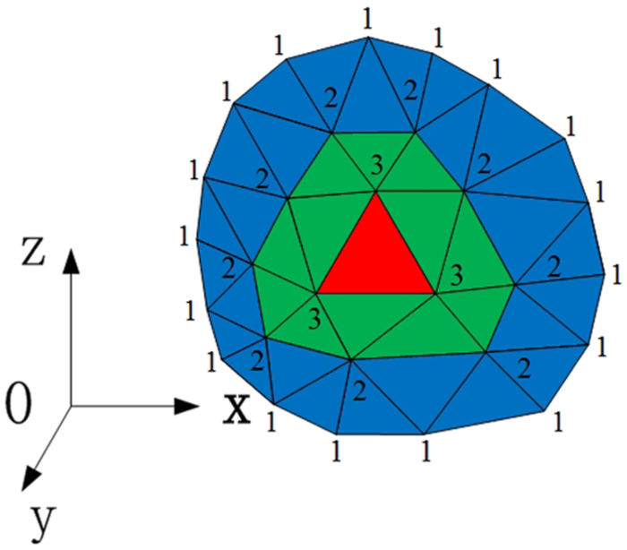
The schematic diagram of center triangle indexing.

Coordinate transforming principle

In order to describe the coordinate transforming principle, a figure is presented as shown in Figure 3.

Figure 3.

The schematic diagram of coordinate transforming: (a) an arbitrary triangle, (b) the triangle after translating, (c) m vector, and (d) the triangle after rotating.

As shown in Figure 3(a), there is an arbitrary triangle ΔP₁P₂P₃ in space rectangular coordinate system 0-xyz and its vertex coordinates are P₁(x₁, y₁, z₁), P₂(x₂, y₂, z₂), and P₃(x₃, y₃, z₃), respectively.

First, an orthogonal matrix can be preset, denoted as ${\mathbf{R}}_1=[\begin{array}{ccc}\hfill {\mathbf{R}}_{\mathrm{x}}\hfill & \hfill {\mathbf{R}}_{\mathrm{y}}\hfill & \hfill {\mathbf{R}}_{\mathrm{z}}\hfill \end{array}{]}^{\mathrm{T}}=\left[\begin{array}{ccc}\hfill r_{1x}\hfill & \hfill r_{2x}\hfill & \hfill r_{3x}\hfill \\ \multicolumn{1}{c}{r_{1y}}& \hfill r_{2y}\hfill & \hfill r_{3y}\hfill \\ \multicolumn{1}{c}{r_{1z}}& \hfill r_{2z}\hfill & \hfill r_{3z}\hfill \end{array}\right]$ . The local coordinate system 0′-x′y′z′ can be established by three vertices, as shown in Figure 3(a). Presetting ${\mathbf{R}}_{\mathrm{x}}=[\begin{array}{ccc}\hfill r_{1x}\hfill & \hfill r_{2x}\hfill & \hfill r_{3x}\hfill \end{array}]=\frac{{\mathbf{P}}_1{\mathbf{P}}_2}{\left|{\mathbf{P}}_1{\mathbf{P}}_2\right|}$ , ${\mathbf{R}}_{\mathrm{y}}=[\begin{array}{ccc}\hfill r_{1y}\hfill & \hfill r_{2y}\hfill & \hfill r_{3y}\hfill \end{array}]=\frac{{\mathbf{P}}_1{\mathbf{P}}_2\times {\mathbf{P}}_1{\mathbf{P}}_3}{|{\mathbf{P}}_1{\mathbf{P}}_2\times {\mathbf{P}}_1{\mathbf{P}}_3|}$ , and ${\mathbf{R}}_{\mathrm{z}}=[\begin{array}{ccc}\hfill r_{1z}\hfill & \hfill r_{2z}\hfill & \hfill r_{3z}\hfill \end{array}]={\mathbf{R}}_{\mathrm{y}}\times {\mathbf{R}}_{\mathrm{x}}$ , these three vectors can be regarded as three axes 0′x′, 0′y′, and 0′z′ in the local coordinate system.

In order to facilitate the subsequent calculations, the local coordinate system should be rewritten in homogeneous coordinate system form by usage, denoted as ${\mathbf{R}}_2=\left[\begin{array}{cccc}\hfill r_{1x}\hfill & \hfill r_{2x}\hfill & \hfill r_{3x}\hfill & \hfill 0\hfill \\ \multicolumn{1}{c}{r_{1y}}& \hfill r_{2y}\hfill & \hfill r_{3y}\hfill & \hfill 0\hfill \\ \multicolumn{1}{c}{r_{1z}}& \hfill r_{2z}\hfill & \hfill r_{3z}\hfill & \hfill 0\hfill \\ \multicolumn{1}{c}{0}& \hfill 0\hfill & \hfill 0\hfill & \hfill 1\hfill \end{array}\right]$ . ²⁸ The translation matrix can be denoted as $\mathbf{T}(-x_1,-y_1,-z_1)=\left[\begin{array}{cccc}\hfill 1\hfill & \hfill 0\hfill & \hfill 0\hfill & \hfill -x_1\hfill \\ \multicolumn{1}{c}{0}& \hfill 1\hfill & \hfill 0\hfill & \hfill -y_1\hfill \\ \multicolumn{1}{c}{0}& \hfill 0\hfill & \hfill 1\hfill & \hfill -z_1\hfill \\ \multicolumn{1}{c}{0}& \hfill 0\hfill & \hfill 0\hfill & \hfill 1\hfill \end{array}\right]$ and the translation result is shown in Figure 3(b). The angles between z′-axis with x-, y-, and z-axis can be denoted as α, β, and γ.

By rotating a certain angle, the two coordinate systems lap over each other. The z′-axis in Figure 3(b) and m vector in Figure 3(c) represent an identical oblique line. Two rotation matrixes can be denoted as R(θ) and R(ω)

$$R(\theta )=\left[\begin{array}{cccc}\cos \theta & \sin \theta & 0& 0\\ -\sin \theta & \cos \theta & 0& 0\\ 0& 0& 1& 0\\ 0& 0& 0& 1\end{array}\right],R(\omega )=\left[\begin{array}{cccc}\cos \omega & 0& -\sin \omega & 0\\ 0& 1& 0& 0\\ \sin \omega & 0& \cos \omega & 0\\ 0& 0& 0& 1\end{array}\right]$$

The combinatorial transformation matrix can be denoted as Y

$$Y=R(\theta )\cdot R(\omega )\cdot T(-x_1,-y_1,-z_1)=\left[\begin{array}{cccc}\cos \theta \cos \omega & \sin \theta & -\cos \theta \sin \omega & -x_1\\ -\sin \theta \cos \omega & \cos \theta & -\sin \theta \sin \omega & -y_1\\ \sin \omega & 0& \cos \omega & -z_1\\ 0& 0& 0& 1\end{array}\right]$$

(3)

Comparing Figure 3(b) with Figure 3(c), the direction cosines of z′-axis (m vector) are $m_1=\cos \alpha$ , $m_2=\cos \beta$ , and $m_3=\cos \gamma$ , respectively.

Analyzing the Figure 3(c), the following formulas can be calculated

$$\{\begin{array}{c}\hfill \cos \omega =\cos \gamma \hfill \\ \multicolumn{1}{c}{\sin \omega =\sqrt{{\cos }^2\alpha +{\cos }^2\beta }}\\ \multicolumn{1}{c}{\cos \theta =\cos \alpha /\sqrt{{\cos }^2\alpha +{\cos }^2\beta }}\\ \multicolumn{1}{c}{\sin \theta =\cos \beta /\sqrt{{\cos }^2\alpha +{\cos }^2\beta }}\end{array}$$

(4)

Substituting cos ω, sin ω, cos θ, and sin θ into equation (7), the final form of combinatorial transformation matrix Y can be presented as follows

$$\mathbf{Y}=\left[\begin{array}{cccc}\hfill \frac{\cos \alpha \cos \gamma }{\sqrt{{\cos }^2\alpha +{\cos }^2\beta }}\hfill & \hfill \frac{\cos \beta }{\sqrt{{\cos }^2\alpha +{\cos }^2\beta }}\hfill & \hfill -\cos \alpha \hfill & \hfill -x_1\hfill \\ \multicolumn{1}{c}{\frac{-\cos \beta \cos \gamma }{\sqrt{{\cos }^2\alpha +{\cos }^2\beta }}}& \hfill \frac{\cos \alpha }{\sqrt{{\cos }^2\alpha +{\cos }^2\beta }}\hfill & \hfill -\cos \beta \hfill & \hfill -y_1\hfill \\ \multicolumn{1}{c}{\sqrt{{\cos }^2\alpha +{\cos }^2\beta }}& \hfill 0\hfill & \hfill \cos \gamma \hfill & \hfill -z_1\hfill \\ \multicolumn{1}{c}{0}& \hfill 0\hfill & \hfill 0\hfill & \hfill 1\hfill \end{array}\right]$$

(5)

By utilizing the combinatorial transformation matrix Y, an arbitrary triangle in the space would be transformed into a specific plane.

Initial flattening method

In this article, the number of triangle limiting the node transforming would be defined as flattening constraint degree of the node to reflect the flattening characteristic during the flattening process. According to this definition, the flattening constraint degree of the node can be divided into three situations.

Situation 1

The triangles T and T₁ represent the arbitrary flattened and unflattened triangles in the space shown in Figure 4(a). The triangles $T\prime$ and $T_1\prime$ are their corresponding flattening result in the plane shown in Figure 4(b). The position of node p₃ can be determined by the intersection of two circles whose centers and radii are nodes p₁, p₂ and r₁₃, r₂₃, respectively, where $r_{13}=\left|P_1{P}_3\right|$ and $r_{23}=\left|P_2{P}_3\right|$ . It can be found the flattening constraint degree of node P₃ is equal to 1. The triangle can be flattened without deformation and there is no elastic deformation energy during the flattening process. For undevelopable surface, this situation rarely occurs. Therefore, it is very significative to study the situation that the flattening constraint degree of the node is greater than 1.

Figure 4.

Situation 1 of flattening constraint degree: (a) an arbitrary triangle and (b) the triangle after flattening.

Situation 2

As shown in Figure 5(a), the flattening constraint degree of node P₃ is equal to 2. The node P₃ can be transformed into the plane, respectively, in the triangles T₁ and T₂ under the Situation 1. The two nodes $p{\prime }_3(x_1,y_1)$ and $p_3^{″}(x_2,y_2)$ can be obtained, named as fake-node, as shown in Figure 5(b). On the basis of these two fake-nodes, the position of only node p₃(x, y) will be determined, where x = (x₁ + x₂)/2 and y = (y₁ + y₂)/2. Thus, the triangles T₁ and T₂ can be flattened easily, denoted as triangles $T_1\prime$ and $T{\prime }_2$ shown in Figure 5(b). Under this kind of situation, the triangle would be flattened with deformation, such as the edge stretching or compressing and also overlaps or cracks come into being. Meanwhile, there exists the elastic deformation energy during the flattening process.

Figure 5.

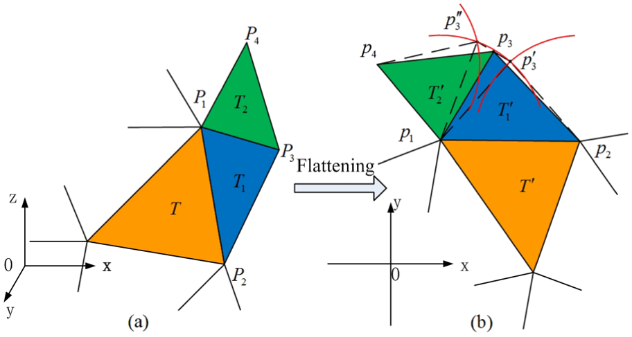
Situation 2 of flattening constraint degree: (a) an arbitrary triangle and (b) the triangle after flattening.

Situation 3

Extending to a more general situation shown in Figure 6(a), the flattening constraint degree of node P₃ is equal to 3. There are three fake-nodes in Figure 6(b), denoted as $p{\prime }_3(x_1,y_1)$ , $p_3^{″}(x_2,y_2)$ , and $p_3^{‴}(x_3,y_3)$ . Figure 5(c) shows the partially enlarging pattern of topology relation of these three fake-nodes. Connecting these three fake-nodes sequentially according to the right-hand rule forms a triangle $p_3^{\prime }{p}_3^{″}{p}_3^{‴}$ . The geometric center p₃(x, y) of this triangle would be regarded as the only position of node P₃ in this article. Thus, the triangles T₁, T₂, and T₃ in the space can be flattened to the plane corresponding to triangles $T_1\prime$ , $T_2\prime$ , and $T_3\prime$ shown in Figure 6(b).

Figure 6.

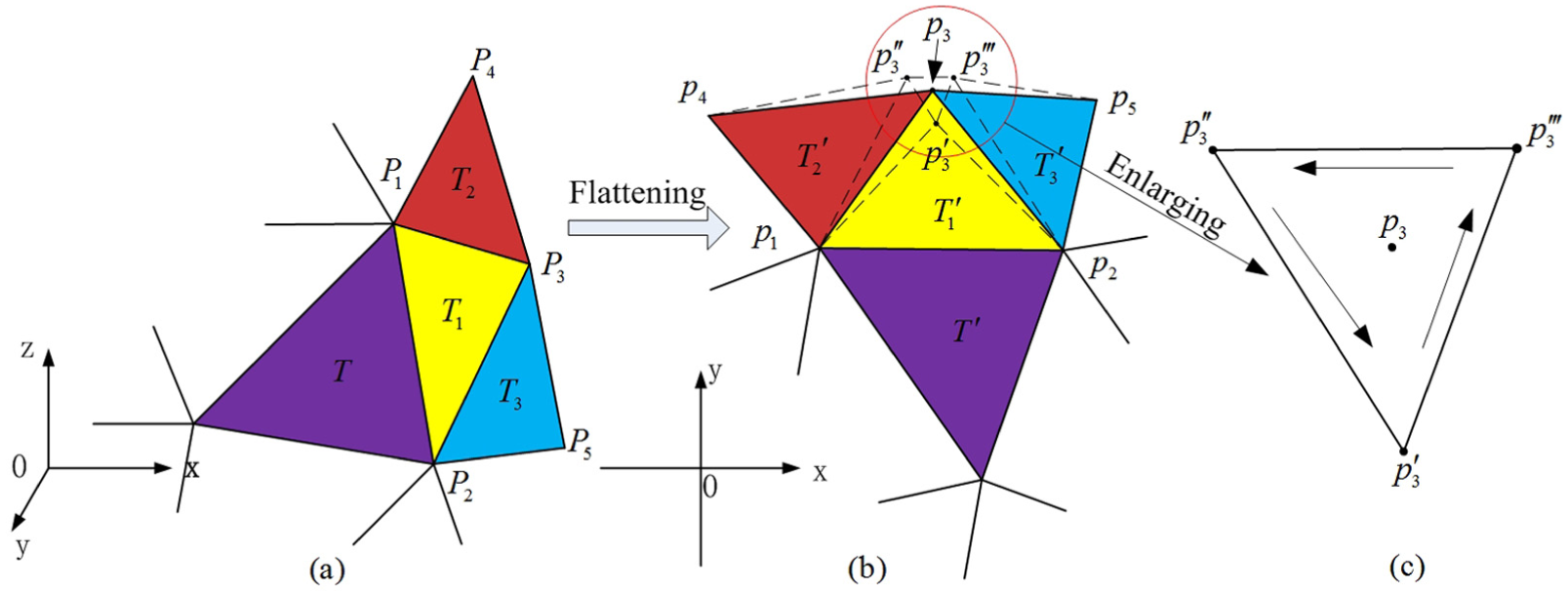
Situation 3 of flattening constraint degree: (a) an arbitrary triangle, (b) the triangle after flattening, and (c) the drawing of partial enlargement.

A method to calculate the geometric center p(x, y) of nonself-intersectant closed polygon is presented. Hypothetically, the nonself-intersectant closed polygon has n $(n\ge 3)$ vertices and its area S can be calculated as follows

$$S=\frac{1}{2}\sum _{i=0}^{n-1}(x_i{y}_{i+1}-x_{i+1}{y}_i)$$

(6)

The geometric center p(x, y) of nonself-intersectant closed polygon can be calculated as follows

$$\{\begin{array}{c}\hfill p_x=\frac{1}{6S}{\sum }_{i=0}^{n-1}(x_i+x_{i+1})(x_i{y}_{i+1}-x_{i+1}{y}_i)\hfill \\ \multicolumn{1}{c}{p_y=\frac{1}{6S}{\sum }_{i=0}^{n-1}(y_i+y_{i+1})(x_i{y}_{i+1}-x_{i+1}{y}_i)}\end{array}$$

(7)

Although the initial flattening result is quite rough, the triangular mesh topology has the same geometrical topology structure in the space domain and plane domain.

Optimizing model

In order to optimize the initial flattening result, a planar spring–mass model is presented in this section.

The planar spring–mass model can be described as follows: the nodes and edges of the initial flattening result can be treated as particles and springs, respectively. Then the physical quantities of the model correspond to the geometric quantities of graphics, such as the quality of particles closely correlates with the area of triangle, and the elastic force is associated with edge difference of triangle flattening pre and post. The difference is considered to be a tension or compression for springs in the model. ²⁹ As shown in Figure 7, the particles p_i and p_j are connected with springs. If the edge p_ip_j on the planar triangular mesh is shorter than the corresponding edge on the spatial triangular mesh, it can be assumed that there exists thrust force between them such as p₀ and p₁; otherwise, there exists tension force such as p₀ and p₅.

Figure 7.

Planar spring–mass model.

Assume that the surface mass is concentrated on each particle. Thus, the mass m_i of particle p_i can be calculated as follows

$$m_i=\frac{\rho }{3}\sum _{j=1}^n{S}_j$$

(8)

where ρ is the area density of the surface, S_j is the area of jth triangle containing the particle p_i, and n is the total number of triangles containing the particle p_i.

The resultant force F _i on a single particle p_i can be defined as follows

$${\mathbf{F}}_i=\sum _{j=1}^{n}k(\left|p_i{p}_j\right|-\left|P_i{P}_j\right|){\mathbf{N}}_{p_i{p}_j}$$

(9)

where k is the elastic coefficient, $|p_i{p}_j|$ is the current distance between particles p_i and p_j on the planar triangular mesh, $|P_i{P}_j|$ is the distance counterpart on the spatial triangular mesh, and ${\mathbf{N}}_{p_i{p}_j}$ is the unit vector pointing from p_i to p_j.

The simplified Lagrange equation can be adopted to describe the motion process of particles in the model ³⁰

$$\mathbf{M}\stackrel{··}{q}+\mathbf{K}q=0$$

(10)

where q is the position of particle, M and K are the mass matrix and stiffness matrix of the spring–mass model, respectively, and K q is the elastic force defined in equation (9).

The Euler method can be applied to solve equation (10). ³¹ When time increment Δt is short enough, the acceleration of the particle is regarded as a constant and then the balance of the whole model will be made up of the balance for each single particle. For arbitrary particle p_i, equation (10) can be rewritten as follows

$$\{\begin{array}{c}\hfill {\stackrel{··}{q}}_i^t=\frac{{\mathbf{F}}_i^t}{m_i}\hfill \\ \multicolumn{1}{c}{{\stackrel{·}{q}}_t^{t+\Delta t}={\stackrel{·}{q}}_i^t+\Delta t{\stackrel{··}{q}}_i^t}\\ \multicolumn{1}{c}{q_i^{t+\Delta t}=q_i^t+\Delta t{\stackrel{·}{q}}_i^t+\frac{\Delta t^2}{2}{\stackrel{··}{q}}_i^t}\end{array}$$

(11)

where ${\stackrel{··}{q}}_i^t$ is the acceleration of particle p_i at time t; ${\stackrel{·}{q}}_i^t$ , ${\stackrel{·}{q}}_i^{t+\Delta t}$ and $q_i^t$ , $q_i^{t+\Delta t}$ are the velocity and position of particle p_i at time t and t + Δt, respectively. It is necessary to state that the ρ in equation (8) and the k in equation (9) are just the weighting factors to make the model more realistic and their values associate with the material properties of sheet metal.

However, by studying equation (11), it can be found that the velocity of particle p_i at time t + Δt is seriously influenced by the velocity at time t. With the accumulation of velocity and the inertia of the particle motion, the particle would oscillate at the equilibrium position, which would bring about divergence for iterative process.

In order to tackle those limitations, the inertia of the particle can be ignored; ³² in other words, the particle moves at a uniform velocity from time t and t + Δt. Therefore, equation (11) can be simplified as follows

$$\{\begin{array}{c}\hfill {\stackrel{··}{q}}_i^t={\mathbf{F}}_i^t/m_i\hfill \\ \multicolumn{1}{c}{{\stackrel{·}{q}}_t^{t+\Delta t}=\Delta t{\stackrel{··}{q}}_i^t}\\ \multicolumn{1}{c}{q_i^{t+\Delta t}=q_i^t+\Delta t{\stackrel{·}{q}}_i^{t+\Delta t}}\end{array}$$

(12)

In order to measure the error of the flattening result, the classical error measure rules are adopted in this article. ³³ The area error E_S and length error E_L are defined as follows

$$\{\begin{array}{c}\hfill E_S=\frac{\sum |S_i-S_i\prime |}{\sum S_i}\hfill \\ \multicolumn{1}{c}{E_L=\frac{\sum |L_i-L_i\prime |}{\sum L_i}}\end{array}$$

(13)

where S_i and L_i are the actual edge length and area of one triangle on the spatial mesh surface, respectively; $S_i\prime$ and $L_i\prime$ are the edge length and area of its corresponding triangle on the flattened mesh surface, respectively.

In order to obtain an effective and meaningful flattening result, the following restricted conditions should be satisfied

$$\{\begin{array}{c}\hfill E_S\le {\epsilon }_S\hfill \\ \multicolumn{1}{c}{E_L\le {\epsilon }_L}\end{array}$$

(14)

where ε_S and ε_L are the tolerance of area error and length error, respectively.

Because the shape of the triangle is constantly changing, the mass matrix and the elastic force are also changing constantly. The iterative process has complicated nonlinear features. The calculation steps are shown as follows:

• Step 1. Preset the time increment Δt, the tolerance of error ε_S and ε_L, and the maximum iterations ε_i.

• Step 2. Calculate the mass m_i of each particle and the resultant force F _i on each single particle.

• Step 3. Solve the new physical parameters of particles through equation (12).

• Step 4. Calculate the area error E_S and length error E_L through equation (13).

• Step 5. If $E_S\le {\epsilon }_S$ , $E_L\le {\epsilon }_L$ or the iterations are greater than ε_i, exit the iteration; or go to Step 2.

With the optimizing process completed, the particles and springs achieve a global stability state and the final flattening result of the original surface can be obtained.

Flowchart of the flattening method

According to the above description, the proposed flattening method can be coded easily on the computer, and the flowchart can be summarized as shown in Figure 8.

Figure 8.

Flowchart of the flattening method.

Simulation examples and discussion

Based on the above technologies, the flattening system for sheet metal with free-form surface has been developed through integration of Microsoft visual studio 2008 and OpenGL. All the examples are executed on a Core-i5 2.53G PC. The simulation results are shown in Figures 9–11, and the comparison results are listed in Table 1.

Figure 9.

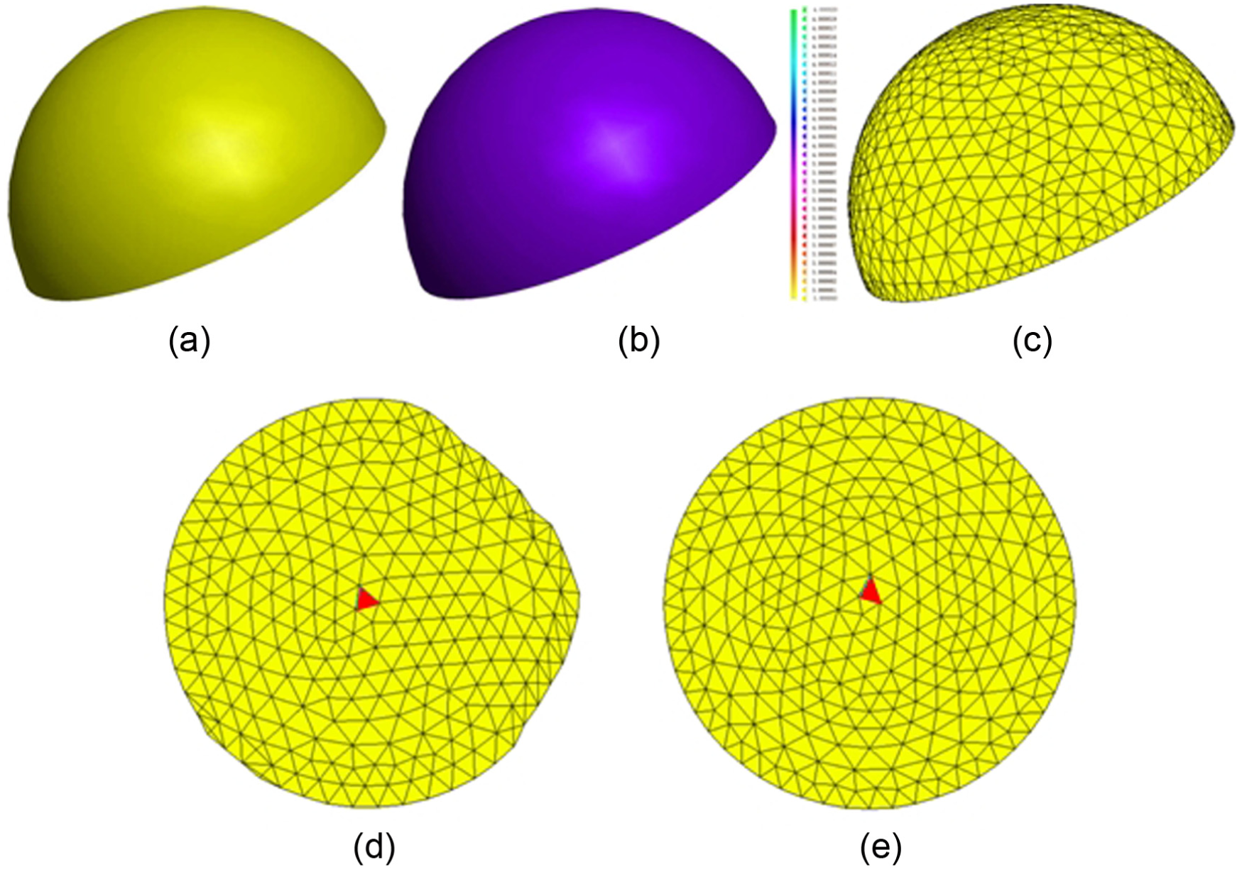
A hemisphere flattening example: (a) initial free-form surface, (b) Gaussian curvature nephogram, (c) meshed surface, (d) initial flattening result, and (e) optimizing result.

Figure 10.

A rotational part flattening example: (a) initial free-form surface, (b) Gaussian curvature nephogram, (c) meshed surface, (d) initial flattening result, and (e) optimizing result.

Figure 11.

A thin sheet flattening example: (a) initial free-form surface, (b) Gaussian curvature nephogram, (c) mesh quality Δ₁ = 0.65, (d) optimizing result, (e) mesh quality Δ₁ = 0.95, and (f) optimizing result.

Table 1.

Comparison results.

Example	Gaussian curvature	Mesh quality	Node no.	Triangle no.	Result	ES (%)	EL (%)
A hemisphere flattening	4e−4	0.91	690	1272	Initial flattening result	1.532	1.467
					Optimizing result	0.463	0.113
A rotational part flattening	Max 3.15e−4	0.93	834	1462	Initial flattening result	2.874	5.627
	Min −6.86e−4				Optimizing result	1.365	1.014
A thin sheet flattening	Max 0	0.65	548	967	Optimizing result	5.670	9.631
	Min −2.53e−6	0.95	1365	2368		1.647	2.362

The flattening results of a hemisphere are shown in Figure 9. In fact, the hemisphere is a typical undevelopable surface and its Gaussian curvature is a constant. The simulation results show that the flattening quality can be improved greatly when the planar spring–mass model is applied. After optimizing, the area error E_S can be reduced from 1.532% to 0.463% and the length error E_L can be reduced from 1.467% to 0.113%. Obviously, the flattening quality of hemisphere is improved greatly.

The flattening results of a rotational part are shown in Figure 10. The rotational part is more complicated than the hemisphere and its Gaussian curvature is not a constant as shown in Figure 10(b). The target surface is first meshed with 834 nodes and 1462 triangles, shown in Figure 10(c). Applying the planar spring–mass model in the example, the area error E_S is reduced from 2.874% to 1.365% and the length error E_L is reduced from 5.627% to 1.014%.

In order to verify the influence of mesh quality on the fattening result, a thin sheet flattening example is provided and the flattening results of a thin sheet are shown in Figure 11. From the Gaussian curvature nephogram shown in Figure 11(b), the target surface is a local undevelopable surface. The surface is divided into two kinds of meshes in which the quality measuring values of the triangular mesh surface are Δ₁ = 0.65 and Δ₂ = 0.95. Comparison results indicate that the flattening quality of second kind condition is better than the first.

The interface of the flattening system for sheet metal with free-form surface is shown in Figure 12. The system mainly has three tool bars: tool bar for flattening, tool bar for data exchanging, and tool bar for view transforming module.

Figure 12.

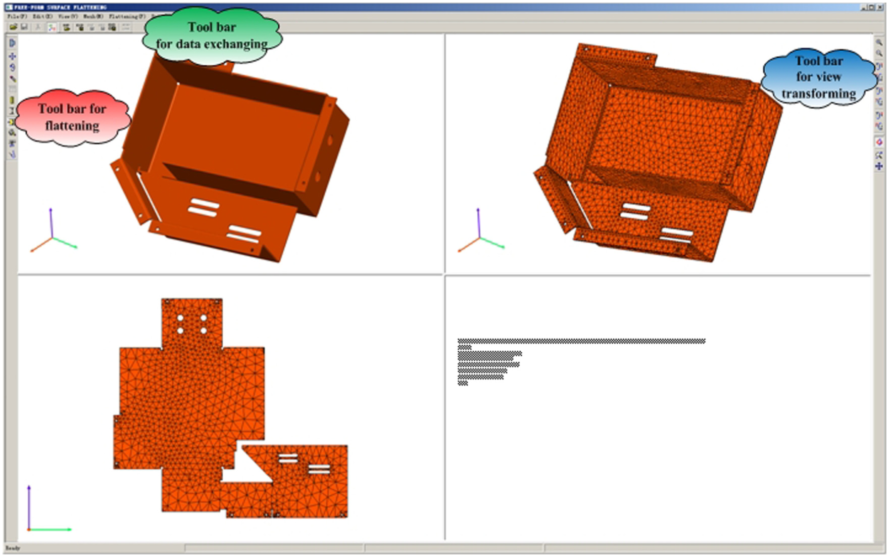
The prototype system interface.

Conclusion and future work

A flattening system for sheet metal with free-form surface was designed and implemented to improve the flattening quality of sheet metal. The framework and its key technologies of the proposed system were elaborated. Finally, three examples were provided and the proposed system was proved feasible and efficient.

In future studies, the authors plan to investigate some improvements for the proposed system such as considering the material property of sheet metal and establishing a better optimizing model. In addition, the applications of the proposed system in mechanical engineering are worth further study for the authors.