Fault diagnosis of rotating machines for rail vehicles based on local mean decomposition—energy moment—directed acyclic graph support vector machine

Abstract

In order to accurately perform fault diagnosis of key rotating machines of rail vehicles, a new method for diagnosis was proposed, based on local mean decomposition—energy moment—directed acyclic graph support vector machine. The vibration signals of rotating machines were decomposed by local mean decomposition to obtain the signal components, and then energy moment is calculated for each state feature component for feature extraction. For state identification, the directed acyclic graph support vector machine is established, multiple classical support vector machine were trained, and then multi-state identification was completed using directed acyclic graph support vector machine. The proposed method was tested on a train rolling bearing. Experimental results show that the method has nearly 95% identification accuracy and verified the feasibility and advantages of this method.

Introduction

A bearing, gear set, and other rotating machines are the key components to support normal rail vehicle operation. Once a fault occurs, it seriously affects the safety of trains and can even cause a fatal accident. Consequently, the precise fault diagnosis of rotating machines has important significance to guarantee the stable operation of the train. According to statistics, rotating machines have the highest failure rate and the most easily damaged parts of modern mechanical equipment. For example, 80% of the rolling bearing cannot reach its service life.^1,2 Therefore, to ensure the vehicle system is working efficiency, and reduce operation and maintenance costs, it is necessary to implement fault diagnosis and condition monitoring accurately for the critical rotating machines.

The traditional fault diagnosis method is mainly through the collected signal in the time domain and frequency domain analysis. Some faults can be diagnosed by detecting the characteristic frequency of different faults. However, the influence of the non-linear factors on sensor signals such as friction, rotational speed, varying load, and stiffness in the rotating machinery operation reduces the diagnosis accuracy of such traditional methods, and they may not satisfy the site requirements. ³ Therefore, modern fault diagnosis methods in recent years are mostly through the processing of sensor signals to extract features and a training identifier by the supervised method on the basis of the feature to complete the fault diagnosis.

With regard to feature extraction, local mean decomposition (LMD) is a new adaptive non-stationary signal processing method. The complicated sensor signal can be decomposed into multiple product functions (PFs) by the high- and low-frequency components. Each PF component is a single amplitude modulation–frequency modulation (AM-FM) signal. The LMD decomposition process is mild, and it can save abundant frequency and envelope information. ⁴ Compared to the widely used wavelet decomposition and empirical mode decomposition method, LMD method has a better performance in inhibiting the endpoint effect, reducing the number of iterations and reserving local information integrity of the signal. ⁵ When rotating machinery faults, the energy distribution within different frequency bands of the signal is not the same. The fault state can be determined by calculating the energy moment (EM) of each component by obtaining PF components of different frequency ranges based on LMD decomposition. In view of this, this article puts forward a method to extract feature based on LMD and EM.

Support vector machine (SVM) classification has superior performance and high computational efficiency for calculating the identifier training on the basis of the extracted features. It not only has good learning ability for small samples but also good generalization ability and can avoid being trapped into local minima effectively. ⁶ It is also characterized by fast calculation speeds without the need to provide approximate accuracy. ⁷ So, it can solve the problems such as small sample and uneven distribution. In addition, there are many successful fields of diagnosis and prediction experiences.^8,9 Therefore, based on the classical SVM, the directed acyclic graph support vector machine (DAGSVM) method was used in multiple classification problems in rotating machinery fault diagnosis.

In this article, a new method for diagnosis based on LMD-EM-DAGSVM was proposed. The manuscript is organized as follows: first, feature extraction method based on the state of LMD and EM is introduced; second, DAGSVM multiple classifiers’ basic principles are given; again, fault diagnosis process is given in detail based on the LMD-EM-DAGSVM method; then, an experiment of train key components for rolling bearing was applied to test the method; Finally, a summary and discussion on future research direction are given.

Feature extraction by LMD-EM

LMD

LMD is a time-frequency analysis method which was proposed by JS Smith ⁵ in 2005. It is not bound by Fourier transformation restrictions and can select frequency bands adaptively according to the vibration signal characteristics and determine signal resolutions of different frequency bands. LMD is suited to analyze the multi-component non-linear and non-stationary signals caused by rotary machinery faults, because it optimizes the signal analysis course and increases the accuracy of useful extracted information. ¹⁰ Recently, some scholars have studied the fault signal feature extraction methods based on LMD, and some methods are proposed, such as the method of combining LMD and order tracking analysis, ¹¹ Fourier transformations are used for the instantaneous frequencies and amplitudes of each component decomposed by LMD, ¹² and an energy operator demodulating approach is based on LMD, ¹³ and calculating envelope spectrum of each component decomposed by LMD ¹⁴ and so on.

The LMD method essence is to isolate pure FM signals and envelope signals from the original signal by iteration, and then multiply the pure FM signals with envelope signals to get a PF component, in which instantaneous frequency is physically meaningful. The multiplication process is repeated until all PF components are extracted.

Considering the decomposition velocity and the accuracy of decomposition results, an LMD method based on cubic spline function was adopted, and the decomposition process is visible in Wang et al. ¹⁵ Figure 1 shows a complex vibration signal x(t) and each PF component PF₁(t) – PF₆(t) of the LMD decomposition and a residual component r(t).

Figure 1.

Vibration signal and its decomposition results.

EM

Multiple PF components from the LMD decomposition contain different frequency bands. When a failure occurs, the frequency energy changes, and energy integration will also change. Signal EM is accumulated in time scales. It can also depict the distribution of the signal energy in different frequency bands and different time periods. Compared to the pure energy, EM can be more sensitive to reflect the change of state. Therefore, the EM calculation of each component can represent changes in the various components and extract the feature of fault state.

EM is defined as follows: assume collecting the original discrete signal x = {x ₁, x ₂, …, x _N} = {x _i}, i = 1, 2, …N, where N is the number of sample points, there is

$$\mathrm{EM}=\sum _{i=1}^N(i·\Delta t){\left|x_i\right|}^2$$

(1)

where $\Delta t$ is the sampling period.

This index has an improved index based on the energy index, which not only takes the amplitude of the vibration signal into account but also considers the amplitude distribution of the signal, so we can reveal the distribution of energy characteristics better.^16,17

State identification by DAGSVM

SVM method was originally designed for binary classification problems. An appropriate multi-class classifier is needed to construct for solving the multi-classification problem, based on the classic SVM. The methods commonly used are one-against-all SVM, one-against-one SVM, and DAGSVM, of which the latter two methods are more suitable for practical applications. However, one-against-one SVM has classification error and rejected points. ¹⁸ DAGSVM puts the idea of the directed acyclic graph in graph theory into the one-against-one SVM and implements one-against-one SVM simplification, thus maintaining higher computational efficiency under certain classification accuracy. Consequently, this article adopts DAGSVM multi-classification method.

For a classification problem with M class data samples, DAGSVM needs to construct the surface between every two types of classification; it has M(M−1)/2 sub-classifiers of completed binary classification. All sub-classifier constituted two-way directed acyclic graphs, including M(M−1)/2 nodes and M leaves. Each node is a sub-classifier and is connected to two nodes (or leaves) of the next layer, from top to bottom. The ith layer has i nodes, that is, the top layer has a node, the M layer M nodes. Classifying an unknown sample begins from the top of the root node (contains two types), and according to the uses of classification results, the next left or right node layer continues classifying until it reaches the leaf of a bottom. The category represented by the leaf is the category of unknown samples. ¹⁹

For example, Figure 2 shows the basic principle of DAGSVM with three categories and three kinds of samples to indentify, A, B, and C.

Figure 2.

DAGSVM basic principle (category = 3).

LMD-EM-DAGSVM fault diagnosis process

The fault diagnosis process was given in detail based on the LMD-EM-DAGSVM method to describe the various technologies:

• Step 1. Collect sensor signal data of each state (including the normal state and various fault states).

• Step 2. Use LMD to decompose the acquired sensor signal. If data samples are too large, in order to guarantee the execution efficiency of the algorithm, according to certain time interval, put the data samples segmented, and then use LMD to decompose each segment of data and obtain the PF components of each segment of data.

• Step 3. Record this minimum number of the components as the state feature vector dimension, to ensure each state owns the same feature vector dimension. Then, the minimum of components is obtained after calculating each component by decomposition (i.e. to find a minimum component segment after decomposition). For example, if a signal under a certain state is divided into five segments, the 1st, 2nd, 3rd, 4th, and 5th segments are decomposed into 6, 7, 8, 6, and 5 components, respectively, then the minimum value is 5, and only the first 5 components are used for the following calculation with the rest abandoned.

• Step 4. After obtaining the PF components of each signal with the same component number, the EM of each signal as the state feature is calculated according to formula (1).

• Step 5. Mark the state features obtained under different states (e.g. “normal,”“fault A,” and “fault B”), and the state feature vectors are marked as the input of DAGSVM, for training classifier.

• Step 6. Trained classifier can be done as a state identifier. The online fault diagnosis completes the first four steps, puts the feature into the state identifier, and outputs the diagnostic results.

Experiments and results

To verify the validity of this article, an example of rolling bearing, the typical key rotating machinery on the train, was applied to test the algorithm. The fault diagnosis experiment of rolling bearing was performed by collecting the vibration acceleration signal.

Vibration data of this article came from Dr Kenneth A Loparo, Western Reserve University Bearing Data Center, ²⁰ and Figure 3 shows the experimental platform. A complete set of experimental data contains four kinds of bearing vibration data, namely, normal, ball fault, inner race fault, and outer race fault. And the number of each state of the testing bearing is one. The test properties of the 205-2RS JEM SKF bearing model–type deep groove ball bearings are the motor load with 3 hp, rotating speed of 1730 r/min (about 28.8 r/s), driver-side sampling, sampling frequency of 48 kHz, and sampling time of 10 s.

Figure 3.

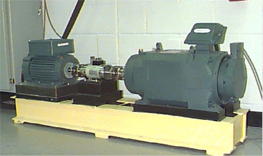
Bearing fault diagnosis experimental platform.

In this article, according to a fixed time interval, the vibration data under four different states are divided into 240 segments, and each segment of data contains 2000 sample points. In the experiment, the state feature of the 240 segment of vibration signal data from the four kinds of state is extracted, obtaining a total of 960 state feature vectors, as the state identifier of train and test samples. And then, the 240 data segments in each state (including the normal, the ball fault, the inner race fault, and the outer race fault) were decomposed by LMD to obtain the PF matrix of each segment. The EM of each PF matrix was computed, and five-dimensional state features were extracted. Finally, DAGSVM was used to achieve the state identification based on the state features. A total of 60% of the state feature vectors were used to train the DAGSVM, and the remaining 40% were the test samples.

For the comprehensive measure algorithm performance, the following two indicators were selected.

1. Classification rate (CR) was used to measure classification accuracy of all samples. CR can be computed by the ratio of all the samples classified correctly and the number of total samples, as shown in formula (2)

   $$\mathrm{CR}=\frac{\mathrm{the}{\mathrm{number}}_{}{\mathrm{of}}_{}{\mathrm{correctly}}_{}{\mathrm{classified}}_{}\mathrm{samples}}{{\mathrm{the}}_{}{\mathrm{number}}_{}{\mathrm{of}}_{}{\mathrm{total}}_{}\mathrm{samples}}$$

   (2)

2. Fleiss kappa statistic (FK) was used for maintaining consistency between quantitative evaluation of identified goals and the classifier output, ²¹ when its value is greater than 0.8, two groups of classification data can be considered almost identical.

Table 1 contains the state of actual status, state feature, and the diagnostic results. They come from five test samples which were randomly selected in each state. It can be seen from the table in the 20 randomly selected test samples that only one fault sample was diagnosed with outer race failure, while the remaining 19 sample diagnostic results are consistent with status. At the same time, as Table 1 shows, the range of feature vectors obtained in different states has a large gap, demonstrating that the LMD-EM can distinguish different states effectively and accurately.

Table 1.

State of actual status, state feature vectors, and the diagnostic results.

State of actual status	State feature	Diagnostic results
Normal	[2.8491, 0.9426, 1.1786, 0.7402, 0.0968]	Normal
Normal	[2.5146, 1.1223, 0.9721, 0.6964, 0.0835]	Normal
Normal	[2.9660, 1.2614, 0.9866, 0.6636, 0.1917]	Normal
Normal	[2.4151, 1.0268, 1.3681, 0.9317, 0.1947]	Normal
Normal	[2.6191, 0.8920, 0.9588, 0.6042, 0.0823]	Normal
Ball fault	[25.1370, 2.6751, 2.7516, 0.3455, 0.1267]	Ball fault
Ball fault	[32.6590, 2.7410, 2.7206, 0.8003, 0.0962]	Outer race fault
Ball fault	[25.8668, 3.1621, 3.1485, 0.7703, 0.1435]	Ball fault
Ball fault	[36.4883, 8.6135, 4.5284, 0.4636, 0.5258]	Ball fault
Ball fault	[28.4829, 3.6662, 2.6679, 0.4071, 0.1176]	Ball fault
Inner race fault	[108.9167, 2.7405, 0.9398, 0.1731, 0.0609]	Ball fault
Inner race fault	[90.4845, 1.9853, 1.1650, 0.2590, 0.0460]	Inner race fault
Inner race fault	[138.6452, 4.0717, 1.0381, 0.3268, 0.0609]	Inner race fault
Inner race fault	[150.0107, 3.9579, 1.1335, 0.1933, 0.0736]	Inner race fault
Inner race fault	[189.3733, 2.6097, 0.9239, 0.3634, 0.0921]	Inner race fault
Outer race fault	[30.0280, 1.5013, 0.4753, 0.2655, 0.0170]	Outer race fault
Outer race fault	[27.1067, 2.5765, 0.7571, 0.5111, 0.1520]	Outer race fault
Outer race fault	[44.2764, 1.5679, 0.7623, 0.1922, 0.0863]	Outer race fault
Outer race fault	[43.5624, 2.2957, 0.8000, 0.1544, 0.0587]	Outer race fault
Outer race fault	[32.0876, 1.8881, 0.5683, 0.4564,0.02777]	Outer race fault

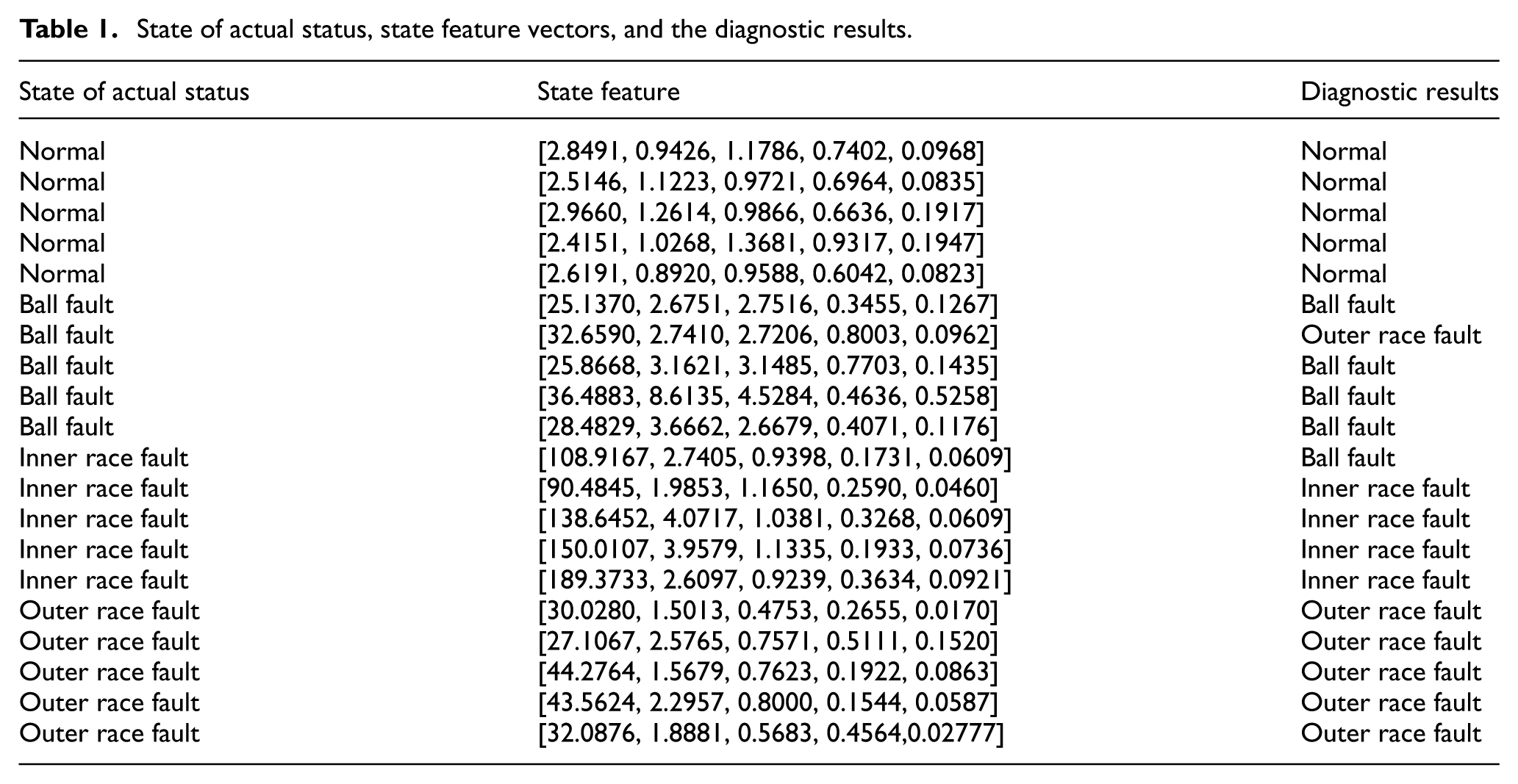
Table 2 gives two index values of training samples and test samples, the CR and the FK. As Table 2 shows, the whole classification accuracy of training samples reached 97.05%, and the FK value is 0.9414. For the test samples, the CR is 0.9467, which corresponds to the FK value of 0.9289. This result shows that the state identifier has been well trained, and the whole diagnostic accuracy of the test samples was high, close to 95%. The results effectively validate the superiority of the proposed fault diagnosis method.

Table 2.

Two index values of training samples and test samples.

Index value	Training samples	Test samples
CR	0.9705	0.9467
FK	0.9414	0.9289

CR: classification rate; FK: Fleiss kappa statistic.

Considering the practical application of the LMD-EM-DAGSVM method, real-time performance should be analyzed. So, the running time of the method was counted. And the running time includes the whole process from inputting original data to outputting state identification results. And it must be noted that the running time contains only the time to complete an online state identification, because the classifier, which is used for online state identification, has been obtained by offline train. The computer hardware environment is Intel(R) Core(TM) 2 Duo CPU E7500 at 2.93 GHz and 2GB RAM. All the codes involved are performed in MATLAB 2012a. After 50-time runs, the average running time is calculated as 0.0494 s. This result indicates that the LMD-EM-DAGSVM method can meet the requirements of field application.

In summary, through experiments, the results of this diagnosis study of rolling bearing showed that this proposed method can diagnose the fault states of rotating machinery accurately, and the real-time performance is good.

Conclusion

According to the accurate fault diagnosis of key rotating machines for rail vehicles, a new method for diagnosis was proposed based on LMD-EM-DAGSVM. EM calculations of vibration signal on the basis of LMD decomposition extracted various state features of rotating machinery accurately and reliably, and the multi-classification method based on DAGSVM identified the various states accurately. An example of train rolling bearing was applied to test the method. Experiments were carried out using the vibration acceleration signal, and the experimental results showed that the proposed method has high identification accuracy and can diagnose different fault states accurately and effectively.