Improvement of airfoil trailing edge bluntness noise model

Abstract

In this article, airfoil trailing edge bluntness noise is investigated using both computational aero-acoustic and semi-empirical approach. For engineering purposes, one of the most commonly used prediction tools for trailing edge noise are based on semi-empirical approaches, for example, the Brooks, Pope, and Marcolini airfoil noise prediction model developed by Brooks, Pope, and Marcolini (NASA Reference Publication 1218, 1989). It was found in previous study that the Brooks, Pope, and Marcolini model tends to over-predict noise at high frequencies. Furthermore, it was observed that this was caused by a lack in the model to predict accurately noise from blunt trailing edges. For more physical understanding of bluntness noise generation, in this study, we also use an advanced in-house developed high-order computational aero-acoustic technique to investigate the details associated with trailing edge bluntness noise. The results from the numerical model form the basis for an improved Brooks, Pope, and Marcolini trailing edge bluntness noise model.

Introduction

Noise generated from wind turbines is known as a barrier for further development of wind energy. The new generation of wind turbines has larger rotor size (e.g. more than 120 m in diameter) which essentially increases the total noise level and causes increased annoyance for nearby living people. As a consequence, noise must be constrained in the design stage when developing new airfoils or rotor blades. High aerodynamic performance has been considered as the key object in the designer’s strategy. However, wind turbines at high tip speed ratio or rotor speed produce high aerodynamic noise. It is clear that airfoils with high aerodynamic performance and low noise emission are of interest. Previous work by Bak et al. ¹ showed the strategy of such an optimum design purpose. There exist different noise prediction models^2–9 which can be coupled to aerodynamic design tools. For example, the TNO Institute of Applied Physics (TNO) trailing edge (TE) noise model^4,5 was applied in the airfoil design process by Bak et al.; ¹ the semi-empirical noise prediction model ³ was applied to optimize a 2.3-MW Siemens machine. ¹⁰

Based on the work of Brooks, Pope, and Marcolini (BPM) ² airfoil noise prediction model, the wind turbine noise prediction tool ³ has shown good agreement with field measurements ¹⁰ for frequencies below 4 kHz while noise at higher frequencies was over-predicted. The predicted high-frequency noise is mainly contributed from TE noise, and more specifically the TE bluntness noise. The TE noise is mainly generated due to the passage of TE vortices from the unstable shear layer on both airfoil suction and pressure sides. Additionally, the TE bluntness noise appears in the case of a nonzero airfoil TE thickness. Since the bluntness thickness is often very small, the vortex shedding behind the blunt TE usually generates high-frequency noise. This issue was studied experimentally by Brooks and Hodgson ¹¹ using a NACA 0012 airfoil. The experimental work provided reliable data for further parametric studies. To improve the model accuracy, a modified formulation to predict TE bluntness noise is proposed in this study based on the results obtained from computational aero-acoustics (CAA) and experiments.

CAA is a more advanced numerical tool that models noise generation from unsteady flows. Efforts have been made in the field of CAA during the last 50 years after the work of Lighthill. ¹² Direct numerical simulation (DNS) becomes available as the vast increase in computer power. Using DNS, however, a very fine mesh and highly accurate schemes both in space and time are needed.^13–16 One of the hybrid numerical method, the flow/acoustic splitting method, was proposed by Hardin and Pope ¹⁷ in 1994. Later on, Shen and Sørensen ¹⁸ remedied the original splitting technique by changing the basic decomposition of the variables. To reduce the growth of hydrodynamic instabilities, some other modifications of the original splitting method were proposed by Ewert and Schröder ¹⁹ and Seo and Moon. ²⁰ The work carried out by Shen and colleagues^21–24 was based on full numerical simulations, with acoustic equations derived directly from the original compressible Navier–Stokes equations. This method is referred to as the flow/acoustic splitting technique. The splitting technique was further developed by Zhu and colleagues^25,26 with the implementation of high-order low-dispersion schemes ²⁷ to the acoustic equations. By using the advanced noise prediction tools,^21–27 the airfoil TE bluntness noise is investigated in this article both numerically and experimentally.

The article is organized as follows. Some progresses of noise measurements and predictions are first presented in section “Progresses on field measurements and model predictions.” In section “CAA approach,” the CAA method is demonstrated to compute a NACA 0012 airfoil with a certain TE bluntness and the solutions are compared to measurements. A NACA 63418 airfoil with two types of TEs is then studied using CAA in order to capture the difference of their noise spectra due to the difference of their TE shape. In section “Semi-empirical modeling,” the BPM model ² is investigated and a modified TE bluntness noise model for wind turbine blade application is proposed. Some conclusions are drawn in the last section.

Progresses on field measurements and model predictions

Noise measurements from megawatt (MW) wind turbines are of great interest for wind turbine developers and customers. Previous measurements from kilowatt (kW) wind turbines ²⁸ do not well represent the case for MW wind turbines due to big variations in rotor size and operational conditions. This section describes very briefly about the acoustic field measurements ²⁹ as well as the model comparisons for a MW wind turbine.

The measurements were carried out at Høvsøre close to the western coast of Jylland in Denmark. The test wind turbine is the one closest to the coast. The two closest neighboring wind turbines were out of operation during the 2 measurement days. During the measurements, the wind speeds were in the range of 3–12 m/s. Not too high wind speeds ensure low background noise from leafs, trees, and waves and so on. With the flat terrain covered by grass, the environmental condition is ideal to carry out noise measurements. The test machine was a Siemens wind turbine. The turbine is variable speed, pitch regulated, and with a rated power above 2 MW.

By using the BPM model combining with the boundary layer parameters calculated for the actual airfoil geometry on the Siemens wind turbine, ²⁹ we can compare our predictions with measurements. As shown in Figure 1, the in-house developed wind turbine noise prediction method takes into account several input parameters: (1) wind turbine geometrical data such as airfoil profiles and twist angles; (2) wind turbine operational data such as wind speed, rotational speed, and pitch setting; and (3) turbulence level and different aerodynamic noise mechanisms.

Figure 1.

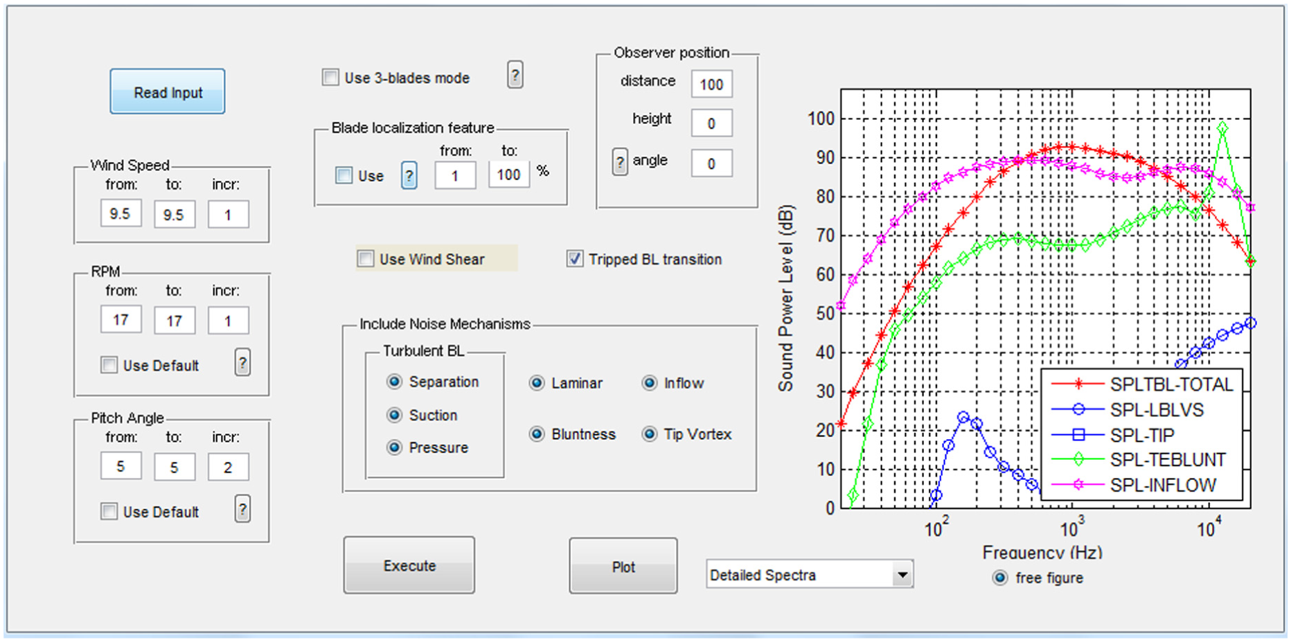
Wind turbine noise prediction software.

As an example, the noise generated from the turbine at various wind speeds is plotted in Figure 2 as a function of shaft rotation speed. Good agreement is clearly seen between the simulation and measurement. The sound power level has almost a linear relation with RPM. A regression analysis indicates that the following relation exists

$$L_w=1.16·\omega +86.12$$

(1)

where L_w is the sound power level in decibels and ω is the main shaft revolution speed given in RPM.

Figure 2.

Noise level against rotational speed.

To check the details at different frequencies, the sound power spectra from the measurement and model simulation are shown together in Figure 3. For the model inputs, the real geometry data are used, for example, the bluntness at various blade stations is obtained directly from measurements. Two sets of measurement data are presented in Figure 3 which was obtained at day 1 and day 2. From the figure, the data are seen to agree well with the simulation for frequencies below 4 kHz. It should be noted that the TE bluntness noise from computation using the BPM model is seen to be the dominant noise source in the high-frequency range. The peak frequency is a function of Strouhal number, Reynolds number, and angle of attack. Since the geometrical input to the prediction model was directly measured from the actual blades, it is evident that the semi-empirical noise prediction model needs be improved. Some CAA computations are carried out in the next section to look more insight into the physics about the bluntness noise problem.

Figure 3.

Weighted one-third octave total noise spectra at an average wind speed of 8 m/s, RPM = 14, pitch = −2°.

CAA approach

CAA methods are much more time-consuming than analytical models. However, CAA methods provide more details of flow and acoustic generation and propagation. In this section, we describe briefly the CAA tool that is used for studying the effects of TE geometry. The CAA method is based on the flow/acoustics splitting technique ¹⁷ which decomposes the compressible Navier–Stokes equations into an incompressible flow part and an acoustic part. The inconsistency of the acoustic formulation was remedied by Shen and Sørensen. ¹⁸ By neglecting the viscous terms, the acoustic equations are written in conservative form as follows

$$\frac{\partial \mathbf{Q}}{\partial t}+\frac{\partial \mathbf{E}}{\partial x}+\frac{\partial \mathbf{F}}{\partial y}+\frac{\partial \mathbf{G}}{\partial z}=\mathbf{S}$$

(2)

where the vectors Q, E, F, G, and S are given in equation (3). In the matrices, the quantities with a superscript (′) indicate acoustic variables and the capital letters U, V, W, and P are the flow variables. The sound speed in equation (3) is calculated at each time step by using $c=\sqrt{\gamma (P+p\prime )/\rho }$ where γ is the specific heat ratio. The acoustic computation can be started at any time after the flow computation is started. At each time level, the flow parameters form the input to the acoustic equations.

$$\begin{array}{c}\mathbf{Q}=\left(\begin{array}{c}\hfill \rho \prime \hfill \\ \multicolumn{1}{c}{\rho u\prime +\rho \prime U}\\ \multicolumn{1}{c}{\rho v\prime +\rho \prime V}\\ \multicolumn{1}{c}{\rho w\prime +\rho \prime W}\\ \multicolumn{1}{c}{\rho \prime }\end{array}\right),\hfill \\ \mathbf{E}=\left(\begin{array}{c}\hfill \rho u\prime +\rho \prime U\hfill \\ \multicolumn{1}{c}{\rho (2\mathrm{Uu}\prime +{u\prime }^2)+\rho \prime U^2+p\prime }\\ \multicolumn{1}{c}{\rho (\mathrm{Vu}\prime +\mathrm{Uv}\prime +u\prime v\prime )+\rho \prime \mathrm{UV}}\\ \multicolumn{1}{c}{\rho (\mathrm{Wu}\prime +\mathrm{Uw}\prime +u\prime w\prime )+\rho \prime \mathrm{UW}}\\ \multicolumn{1}{c}{c^2(\rho u\prime +\rho \prime U)}\end{array}\right),\hfill \\ \mathbf{F}=\left(\begin{array}{c}\hfill \rho v\prime +\rho \prime V\hfill \\ \multicolumn{1}{c}{\rho (\mathrm{Vu}\prime +\mathrm{Uv}\prime +u\prime v\prime )+\rho \prime \mathrm{UV}}\\ \multicolumn{1}{c}{\rho (2\mathrm{Vv}\prime +{v\prime }^2)+\rho \prime V^2+\rho \prime }\\ \multicolumn{1}{c}{\rho (\mathrm{Vw}\prime +\mathrm{Wv}\prime +v\prime w\prime )+\rho \prime \mathrm{VW}}\\ \multicolumn{1}{c}{c^2(\rho v\prime +\rho \prime V)}\end{array}\right)\hfill \\ \mathbf{G}=\left(\begin{array}{c}\hfill \rho w\prime +\rho \prime W\hfill \\ \multicolumn{1}{c}{\rho (\mathrm{Wu}\prime +\mathrm{Uw}\prime +u\prime w\prime )+\rho \prime \mathrm{UW}}\\ \multicolumn{1}{c}{\rho (\mathrm{Wv}\prime +\mathrm{Vw}\prime +v\prime w\prime )+\rho \prime \mathrm{VW}}\\ \multicolumn{1}{c}{\rho (2\mathrm{Ww}\prime +{w\prime }^2)+\rho \prime W^2+p\prime }\\ \multicolumn{1}{c}{c^2(\rho w\prime +\rho \prime W)}\end{array}\right),\hfill \\ \mathbf{S}=\left(\begin{array}{c}\hfill 0\hfill \\ \multicolumn{1}{c}{0}\\ \multicolumn{1}{c}{0}\\ \multicolumn{1}{c}{0}\\ \multicolumn{1}{c}{-\frac{\partial P}{\partial t}}\end{array}\right)\hfill \end{array}$$

(3)

In the following CAA calculations, the incompressible Navier–Stokes equations are solved by the second-order finite volume EllipSys code,^30,31 and the acoustic equations are solved using a sixth-order optimized compact scheme. ²⁶ To reduce the computational cost, only the two-dimensional simulations are carried out. It is assumed that three-dimensional effect is small at low angle of attack, and also the local Reynolds number at the blunt TE is much smaller with the order less than 10⁴. In the first case, we calculate the TE bluntness noise from a NACA 0012 airfoil with a bluntness of about 0.35% chord length. The computational mesh is shown in Figure 4. A two-dimensional structural body-fitted O-mesh is generated with about 150,000 cells. The computational grid in the radial direction is exponentially clustered on the airfoil surface. At the TE, the upper and lower edges are rounded and there is a flat edge between the rounded edges (see Figure 4). Computations are carried out at two Reynolds numbers 1.6 × 10⁶ and 2.8 × 10⁶ at the same angle of attack of 0°. Small-scale turbulence is modeled with a sub-grid scale (SGS) model for large-eddy simulation (LES). In this study, the two-dimensional version of the mixed model developed by Ta Phuoc ³² is used. The eddy viscosity is calculated by using the mixed-scale turbulence model such that ${\nu }_t=C{\left|\overline{\omega }\right|}^{\alpha }{k}^{(1-\alpha )/2}{\Delta }^{(1+\alpha )}$ where ω is the vorticity, k is the turbulent kinetic energy, Δ is an average grid size, and the model constants are C = 0.02 and α = 0.5. For more details, the reader is referred to Ta Phuoc ³² and Sagaut. ³³ The acoustic simulation is started after the flow is fully established. A snapshot of vortex formation at TE is shown in Figure 5(a) for flow at Reynolds number of 1.6 × 10⁶. As expected, the smaller vortex was created behind the blunt TE (vortex A). The larger vortex (vortex B) is generated due to the unsteadiness of laminar to turbulent transition. The small vortex shedding behind the blunt TE is responsible for the tone noise generation. Figure 5(b) shows an instantaneous sound pressure field around the NACA 0012 airfoil. Sound waves are generated mainly at TE. By taking a closer view at the TE, the noise source behind the blunt TE is observed. To quantitatively identify the noise level, further investigation of time history signal is processed. The acoustic pressure signal is stored in a data file at each time step in order to perform fast Fourier transform (FFT) and obtain the noise spectrum. The acoustic pressure signals are selected at 0.05 chords above the TE where the mesh density is very high. To compare CAA results with the measured data, signals at a same distance should be used. Thus, the pressure signals obtained from CAA are scaled to the measurement distances with a decay of $1/\sqrt{r}$ . To get 1/3 octave noise spectra, FFTs are first carried out for the CAA pressure signals after a non-dimensional time of 20 and then the obtained narrow band spectra are transformed into 1/3 octave spectra. The two selected acoustic pressure signals turn out to be quite similar, as can be seen from the sound spectra in Figure 6. The CAA calculations are seen to be able to capture the influence due to TE bluntness. Figure 6(a) and (b) displays together the CAA results and the measurements. ² The TE bluntness noise measurements were performed for a tripped NACA 0012 airfoil with a chord length of 61 cm. The receiver is located at 122 cm above the TE. From the comparisons, it is observed that the blunt TE increases the noise at the high-frequency range and shifts toward higher frequencies with increasing wind speeds.

Figure 4.

Computational mesh for a blunted NACA 0012 airfoil.

Figure 5.

(a) Vortex structure at TE and (b) sound pressure field.

Figure 6.

Calculated 1/3 octave noise spectra compared with the experiments ² at two wind speeds: (a) U = 38.6 m/s and (b) U = 69.5 m/s.

In the next case, we consider a NACA 63418 airfoil with two different TE geometries; see Figure 7. Since NACA 63418 is one of the most used airfoils in modern wind turbine blades, we carry out this computation to determine the influence of changing the TE shape. A similar mesh configuration as the one used for the NACA 0012 airfoil is employed. Flow and acoustic simulations are carried out at zero angle of attack with a Reynolds number of 1.0 × 10⁶. The two TEs differ from each other by means of the TE solid angle Ψ, the angle between lower and upper surfaces near TE. The TE shown in Figure 7(a) is “flat,” compared to the one in Figure 7(b), and the solid angle at TE is estimated such that Ψ ≈ 0° for case (a) and Ψ ≈ 20° for case (b). In Figure 8, two instantaneous plots are shown for the sound pressure contours corresponding to the two types of TE geometry. The sound pressure patterns are basically similar in both cases. However, there is some difference at the very last part of TE where extra noise source appears at the blunt TE but not for the sharp TE. The time history acoustic signals are recorded at 0.05 chords above TE. By making the FFT, the calculated sound spectra are shown in Figure 9 where the effect of TE bluntness is clearly seen. The flat TE (Figure 7(a)) produces distinguishable TE bluntness noise as compared to the sharp one (Figure 7(b)). From the CAA calculations, we conclude that TE bluntness noise exists for airfoils with nonzero bluntness. The sound level is proportional to the thickness and the solid angle Ψ. This solid angle Ψ is discussed in the next section which raises problems when using this semi-empirical model.

Figure 7.

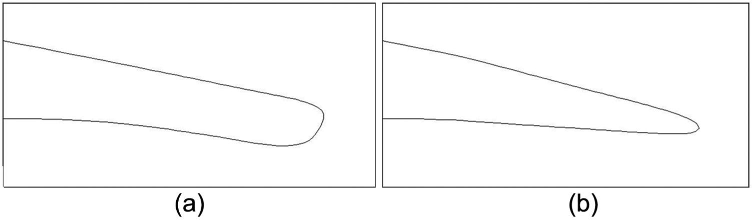
NACA 63418 airfoil with two different trailing edge shapes: (a) Ψ ≈ 0° and (b) Ψ ≈ 20°.

Figure 8.

Sound pressure field of two TE configurations.

Figure 9.

Sound pressure level generated from the airfoil bluntness geometries in Figure 7. Red color corresponds to Ψ ≈ 0°, and blue color corresponds to Ψ ≈ 20°.

Semi-empirical modeling

Semi-empirical noise prediction models are fast and robust which have been widely used for engineering purposes. The airfoil noise prediction model developed by Brooks et al. has been successfully applied to study wind turbine noise^3,10,34 The model captures quite well the broadband noise of a wind turbine. However, it is found that it produces a too high level of TE bluntness noise in several wind turbine noise prediction cases^10,29 (see Figure 3). The prediction using the BPM model is generally in good agreement with measurements, except for the TE bluntness noise, which is highly over-predicted in some cases. The turbine blade employs the NACA 63418 profile in the outer part, which is responsible for the high level of bluntness noise. In the previous section, the TE bluntness noise generated from the NACA 63418 airfoil was simulated by using CAA; see Figure 9. The figure did not show a very high blunt edge noise level, neither with Ψ ≈ 0° nor with Ψ ≈ 20°. It is worth noting that wind turbine blade often have TE shape similar to the one shown in Figure 7(a). Thus, in many cases, a small TE solid angle will be used as an input to the semi-empirical model, for example, Ψ ≈ 0°. Figure 10 shows the prediction using the semi-empirical model with an input of Ψ ≈ 0° which exhibits a very high level of bluntness noise. When this airfoil is employed to construct in the outer part of a wind turbine blade, it predicts similar bluntness noise as seen in Figure 3 where the bluntness noise is over-predicted.

Figure 10.

Sound pressure level at 1 m above the trailing edge of noise generated from a NACA 63418 airfoil with Ψ ≈ 0°.

The semi-empirical TE bluntness noise model of Brooks et al. was developed by scaling the experimental data using only NACA 0012 airfoil. Any kind of TE geometries was simplified by an interpolation between a NACA 0012 airfoil and a flat plate extension. The NACA 0012 airfoil has a solid angle of Ψ ≈ 14° and the flat plate has an angle of Ψ ≈ 0°. Therefore, experiments were carried out for both solid angles and interpolation is applied for any other airfoils with a TE angle between 0° and 14°. A flat plate is mounted at the TE to obtain results at Ψ ≈ 0°. This appears to be a problem for bluntness noise prediction since the TE of wind turbine blades does not have the shape as the flat plate. The use of an interpolation between two angles to represent TE geometry is not universal and had lead to some inaccurate predictions. Also, it will not be convenient to use the model, since the input solid angle has to be measured from a real blade. The idea of modifying the original model is to get the correct boundary layer parameter at the TE and use it as a key parameter. The change in Reynolds number, Mach number, angle of attack, and TE geometry should be well-represented by the boundary layer thickness. The calculation of the boundary layer thickness is performed through XFOIL ³⁵ using a prescribed TE geometry. Using the existing experimental data, ² we fit the sound pressure level and the spectra shape as a function of Mach number, Strouhal number, boundary layer displacement thickness, and so on.

The sound pressure level increases while Mach number increases. The data are plotted in Figure 11(a). From curve-fitting, we get the empirical relation between sound pressure level and Mach number

$$\mathrm{SPL}\propto 10{\log }_{10}{M}^{5.7}$$

(4)

Figure 11.

(a) Sound pressure level as a function of Mach number and (b) shape function at various blunt thicknesses.

Figure 11(b) describes the spectrum shape function where the Strouhal number is defined as

$$\mathrm{St}=\frac{\mathrm{fh}}{U}$$

(5)

where f is frequency, h is the thickness of the blunt TE, and U is the free-stream velocity. The peak Strouhal number is given as

$$S{t}_{peak}=\{\begin{array}{cc}0.149/(1+0.235{(h/{\tilde{\delta }}^{*})}^{-1}-0.0132{(h/{\tilde{\delta }}^{*})}^{-2})& (h/{\tilde{\delta }}^{*}\ge 0.2)\\ 0.1(h/{\tilde{\delta }}^{*})+0.06& (h/{\tilde{\delta }}^{*}<0.2)\end{array}$$

(6)

In equation (6), ${\tilde{\delta }}^{*}$ is the averaged TE displacement thickness of pressure and suction sides. The proportionality between sound pressure level and boundary layer thickness is shown in equation (7)

$$\mathrm{SPL}\propto 10{\log }_{10}\left(\frac{h}{{\tilde{\delta }}^{*}}\right)$$

(7)

A general modified equation is proposed in equation (8) where the Ψ angle is excluded from the amplitude function

$$\begin{array}{c}\multicolumn{1}{c}{\mathrm{SPL}=10{\log }_{10}\left(\frac{2s·h{\sin }^2\left(\frac{\theta }{2}\right){\sin }^2\varphi ·M^{5.7}}{(1+M\cos \theta ){(1+0.2M\cos \theta )}^2·r^2}\right)}\\ \multicolumn{1}{c}{+20(1+M^2){\log }_{10}\left(\frac{h}{{\tilde{\delta }}^{*}}\right)+S_1(\frac{h}{{\tilde{\delta }}^{*}},\frac{\mathrm{St}}{S{t}_{\mathrm{peak}}})+S_2\left(\frac{t}{c}\right)+K_0}\end{array}$$

(8)

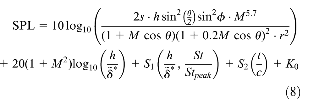
In equation (8), a suggestion for the model constant K₀ is 150 for $h/{\tilde{\delta }}^{*}<0.2$ , otherwise $K_0=150-20(h/{\tilde{\delta }}^{*}-0.2{)}^{0.25}$ , s is the airfoil span, θ and φ are the directivity angles, and S₁ is the shape function that is equivalent to the original G₅ function.

The additional function S₂ gives the correction for the effect of airfoil thickness change along a wind turbine blade

$$S_2=654.43{\left(\frac{t}{c}\right)}^3-652.26{\left(\frac{t}{c}\right)}^2+58.77\left(\frac{t}{c}\right)$$

(9)

For wind turbine case, the influence from the TE bluntness noise becomes less important as the airfoil thickness t/c increases. The forming of the vortex shedding at the blunt TE is favored by an attached flow at TE, where the boundary layer thickness is much smaller than the blunt thickness. At a given angle of attack, the transition points move toward the leading edge as the airfoil thickness increases. The angle of attack is larger at the inner part of the blade that will also produce thicker boundary layer at TE. If the boundary layer thickness becomes larger than the blunt thickness, the flow condition to create bluntness noise becomes poor such as flow over the inner part of a wind turbine blade.

The modified equation (8) is independent of the solid angle and is only a function of the blunt thickness h, the Mach number M, and the averaged boundary layer displacement ${\tilde{\delta }}^{*}$ . In Figure 12, the modified TE bluntness noise model is compared with the previous CAA computation shown in Figure 9. The new TE bluntness noise model predicts much less sound pressure level as compared to the original one, and it is in better agreement with the CAA result.

Figure 12.

Sound pressure level predicted by the new and original blunt noise models, and the CAA computation.

In Figure 13, using the new prediction model, the calculated noise spectrum from a Siemens 2.3-MW wind turbine is compared with the measured data. The prediction method for bluntness noise is modified and the code remains the same for the other noise sources. It is seen that the contribution from bluntness noise is much less with the modified model.

Figure 13.

One-third octave total noise spectra of noise generated from a Siemens 2.3-MW turbine at a wind speed of 8 m/s.

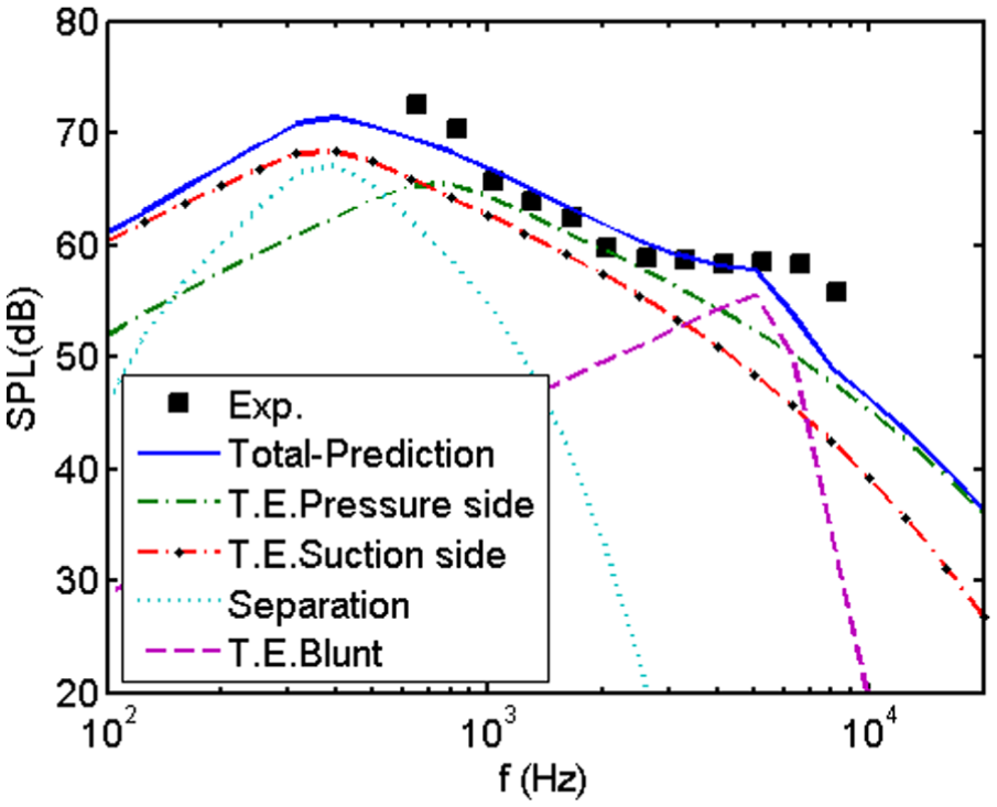
To further verify the empirical relation, we compare the model with some existing experiments from Brooks et al. as shown in Figures 14–16. The new model should be able to fit well with the experimental data as well. In Figure 14, the angle of attack is fixed at 0° and two inflow velocities are simulated. Due to the flow symmetry, the noise spectra of noise from the pressure and suction sides are superimposed and the separation noise does not appear in the plot. The overall noise level and the bluntness noise level are more significant at 70 m/s. In Figure 15, the flow velocity is now fixed at 70 m/s, but different angles of attack are considered. It is observed that airfoil TE bluntness noise decreases when angle of attack increases, which is due to the increase in boundary layer thickness. In Figure 16, we apply the prediction model to a NACA 64418 airfoil. The TE bluntness noise from a NACA 64418 airfoil was observed in the experiments. ³⁶ By assuming a similar bluntness, Figure 16 shows that the model predicts noise emission quite well, as compared with the measured data.

Figure 14.

Sound pressure level from a NACA 0012 airfoil with a chord of 61 cm and a bluntness height of 1.1 mm at an angle of attack of 0° and wind speeds of (a) U = 70 m/s and (b) U = 40 m/s. The experimental data are reproduced from Brooks et al. ²

Figure 15.

Sound pressure level from a NACA 0012 airfoil with a chord of 40.6 cm and a bluntness height of 0.38 mm at a wind speed of 70 m/s and an angle of attack of (a) 0°, (b) 3.9°, and (c) 6.1°.

Figure 16.

Comparison of a NACA 64418 airfoil with chord = 80 cm, angle of attack = 2.7°, U = 60 m/s, and h = 0.8 mm (0.1% chords).

To show the consistency between the original and modified models, comparisons are carried out for TE bluntness noise predictions in the case shown in Figure 14(a). In the original BPM model, the boundary layer thickness at TE is obtained from hotwire measurements. The noise prediction using the modified model is also shown in the same figure which shows the consistency with the original model with hotwire boundary layer data. Furthermore, it is worth noting that the new model is to predict noise from a general airfoil and it is not restricted only for NACA 0012 (Figure 17).

Figure 17.

Comparisons of trailing edge bluntness noise with experiment (selected from Figure 14(a)) using the original BPM model and the modified new model.

Conclusion

TE bluntness noise has been studied in this work. CAA simulations of a NACA 0012 and a NACA 63418 airfoil were carried out for several TE configurations. A semi-empirical noise prediction model has been investigated as well; improvement has been made by using the results from CAA and experiments. The inaccuracy of predicting TE bluntness noise has been remedied with new prediction formula. The model has been validated against the experimental data for both wind turbine airfoil and wind turbine rotor, and good agreements are obtained. The CAA method can provide more physical understanding on noise generation mechanisms, but it is also very time-consuming compared to the engineering models. In the article, it has been shown that CAA can be a useful tool for improving engineering noise prediction models. The general tendency of airfoil TE bluntness noise is observed that (1) TE bluntness edge noise increases with an increase in Mach number, (b) TE bluntness edge noise increases with an increase in blunt thickness, (c) peak frequency decreases with an increase in blunt thickness, (d) TE bluntness noise decreases with an increase in angle of attack, and (e) TE bluntness noise decreases as blade thickness increases.