This article addresses the joint position control of torque-driven robot manipulators under actuators subject to torque saturation. Robots having viscous friction, but without gravity vector, are considered. By assuming a static model for the torque actuator (specifically, a model of nonlinear and non-differentiable hard saturation function), a family of nonlinear proportional–integral–derivative-like controllers is proposed. Lyapunov stability theory is used to establish conditions for local asymptotic stability of the closed-loop system. A notable feature of the proposed controller is that stability conditions do not depend on the saturation levels of the actuators. In addition, an experimental study complements the proposed theory.
Many physical actuators used in control systems have limited capabilities, for example, the amount of force or torque that an electric motor can deliver or the speed at which the rotor can spin.
Actuator saturation occurs when a controller demands a signal greater than the actuator is able to deliver.1 The saturation of the actuators can cause excessive overshoot, long settling time, and sometimes instability.2
Stability for linear systems with bounded inputs has been analyzed, for example, in Suarez et al.,3 Kothare et al.,4 Kothare and Morari,5 and Tarbouriech et al.6 For researches where the stability of nonlinear systems under actuator saturation is analyzed, Robinett et al.7 and Gomes da Silva Jr et al.8 may be mentioned.
Controllers requesting a torque control action limited in amplitude to achieve joint position regulation for torque-driven robot manipulators have been reported in the literature, such as Kelly et al.,9 where a smooth controller and a global asymptotic stability analysis were stated. The standard hard (continuous but non-differentiable) saturation function was considered in Gorez.10 The researches of Zergeroglu et al.11 and Dixon12 proposed adaptive controllers with bounded differentiable saturation functions. In those references, the respective closed-loop system was studied providing conditions for stability of the equilibrium. In Álvarez-Ramírez et al.,13 the standard hard saturation is analyzed obtaining local stability conditions. In Morabito et al.,14 the standard hard saturation was considered and a controller with augmentation anti-windup was used, presenting a global analysis. The work of Kanamori15 considers the standard hard saturation and a local analysis is presented. In Santibañez et al.,16 a continuously differentiable saturation function was used and a global analysis is presented. More recently, in Yokoyama et al.,17 a variable structure controller which uses a switching function to reduce the control action during saturation was proposed.
Other recent approaches to the control of robots and mechanical systems under constrained torque input have been presented in Su et al.,18 which introduced a controller using a smooth saturation function for each component of the controller resembling the structure of a proportional–integral–derivative (PID) controller. A global asymptotical analysis was also presented there. In Izadbakhsh and Fateh,19 the control of electrically driven robots with voltage saturation was addressed. The solution was based on model reference adaptive control. In Su and Swevers,20 a finite time trajectory tracking controller for robots with actuator saturation was proposed. Bounding of the generated control action is guaranteed by means of individuals’ saturations of the proportional and derivative part of the controller and assuming that the desired trajectory is bounded. A sliding mode–based repetitive learning control method for high-precision tracking of robot manipulators with actuator saturation was introduced by Tian and Su.21 Lyapunov’s direct method was employed to prove semiglobal asymptotic tracking.
This article deals with the introduction of a family of controllers for joint position regulation of torque-driven robot manipulators having viscous friction but without gravity vector whose torque-driven actuators are modeled by nonlinear and non-differentiable hard saturation function. Knowledge of the bounds of the parameters of the manipulator is required for controller tuning, but no actuator parameters are needed.
Like in Álvarez-Ramírez et al.,13 Morabito et al.,14 and Yokoyama et al.,17 in the analysis of this article, the hard (non-differentiable) saturation function is considered the torque actuator model.
Most of the controllers in the above-written literature review rely in the selection of gains that depend on the saturation levels of the actuators.
The contribution of this article is a family of controllers inspired by a controller proposed in Kanamori.15 The proposed controller in this article introduces a globally Lipschitz function in the integral action instead of the non-differentiable dead-zone function used by Kanamori’s law. Our study also provides an easy tuning guideline based on explicit bounds of the robot parameters. The proposed family of controllers relies in a rigorous stability analysis. The stability conditions do not depend on the saturation levels of the actuators, but only on a scalar parameter related to the plant parameters but no actuator parameters are needed. Our new control design allows also the addition of an “artificial” hard saturation by programming, which has the aim of providing protection for the actuators. A real-time experimental study in a 2 degree-of-freedom (DOF) manipulator supports the proposed theory. Proofs of properties of the hard (non-differentiable) saturation function are included.
Preliminaries
Notations
Matrices are denoted by bold capital letters, vectors by bold lowercase Latin or Greek letters, is the real vector space of dimension n, is the Euclidean norm of vector . The largest and smallest eigenvalues of a symmetric matrix are expressed by and , respectively.
Robot model
The dynamics of an n-DOF serial revolute joints torque-driven robot manipulator having viscous friction but without gravity vector can be straightforwardly derived from models studied in Sciavicco and Siciliano22 and in Kelly et al.23
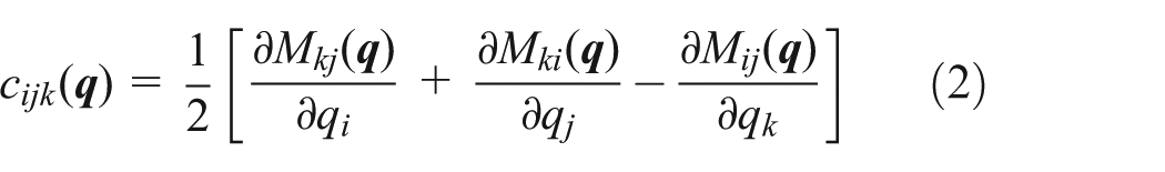
where are the position, velocity, and acceleration, respectively, is a matrix function called inertia matrix, is a diagonal positive definite constant matrix containing viscous friction coefficients, is a matrix function called centrifugal and Coriolis forces matrix and here it is assumed to be obtained using the Christoffel symbols of the first kind , defined as24
where denotes the ijth element of the inertia matrix . Vector is the torque control input. The following properties are used in this article:23
Property 1. The inertia matrix is a symmetric positive definite matrix.
Property 2. , for all and .
Property 3. There exists a positive constant such that .
Assumptions and conventions
With regard to the robot model (1), this article uses the following assumption and convention:
Assumption 1. Position and velocity measurements are available from system (1).
Convention 1. Plant model (1) is associated exclusively to the mechanical structure excluding actuators and sensors (see Figure 1).
Convention 1: The plant model is associated exclusively to the mechanical structure excluding actuators and sensors.
Actuator model
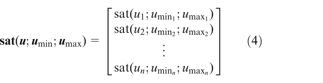
It is assumed that the input to the robot model (1) is a vector function generated by torque type actuators (torque-supply devices) with torque limited capabilities. The input to the robot model (1) is represented by
where is the output of the actuator and
where are the control actions generated by the controller and requested to the corresponding actuators (Figure 2) and , represent the minimum and maximum torque limit saturation levels, respectively, that the ith actuator can safely deliver (see left part of Figure 3).
The output u of the controller is the value requested to the actuator and the output of the actuator is (input to the plant).
Graphs of functions. Left: Saturation function . Right: Dead-zone function .
With regard to vector function in equation (4), it has valuable features summarized in Appendix 1.
Assumption 2. The torque limits and that actuators are able to supply are constant.
In agreement to Assumption 2, the hard saturation function is defined as
where is the independent variable (requested torque) and are the saturation levels constant parameters. So the first argument is the unique independent variable (separated from the function parameters by semicolon symbols).
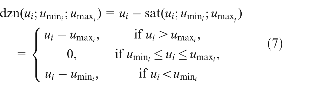
Difference between and defines the dead-zone function
Vector is defined as
The left-hand side of Figure 3 shows the plot of saturation function , while the right-hand side of Figure 3 depicts the dead-zone function .
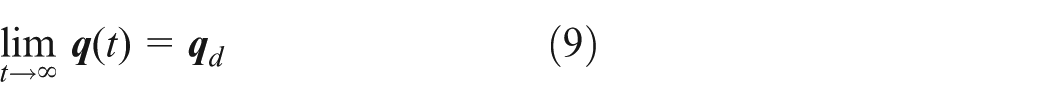
Control objective
The control objective is joint position regulation
where is an arbitrary constant vector.
Proposed control scheme
This article proposes the following family of nonlinear dynamic controllers (PID-like controllers)
where is the joint position error, are arbitrary positive definite constant diagonal matrices. The control law structure in equations (10) and (11) has been motivated from a controller proposed by Kanamori.15 Control law (equations (10) and (11)) can also be seen as a PD control plus nonlinear filtering of position error.
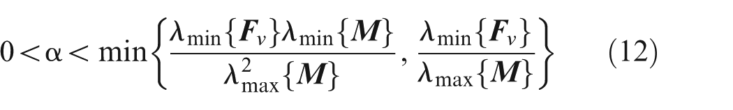
Parameter α of the controller (equations (10) and (11)) is tuning according to
The rationale behind the tuning rule (12) is presented in the next section, where the closed-loop system derived from the robot model (1), actuator model (3), and controller (equations (10) and (11)) is analyzed.
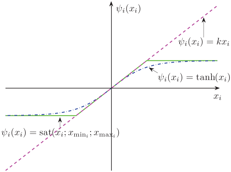
For a vector , function in equation (11) is a continuous vector function having the following structure and properties
where is a globally Lipschitz function satisfying the inequality
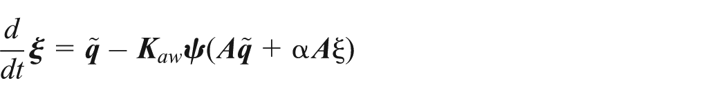
Figure 4 shows a diagram of the proposed family of dynamic controllers (equations (10) and (11)). On the other hand, Figure 5 depicts examples for user-defined Lipschitz function . In Figure 5, (saturation levels), is constant.
Proposed family of nonlinear dynamic controllers (PID-like regulators).
Examples of functions .
There is no claim that the controller nor the control action u are bounded. Nevertheless, the output of the actuator model (3) is bounded.
Analysis
The closed-loop equation with robot model (1), actuator model (3), and proposed control scheme in equations (10) and (11) is
The origin of the state space is the unique equilibrium point of equation (16). To ensure the control objective (equation (9)), in the following, Lyapunov’s direct method is used, as stated in Vidyasagar.25
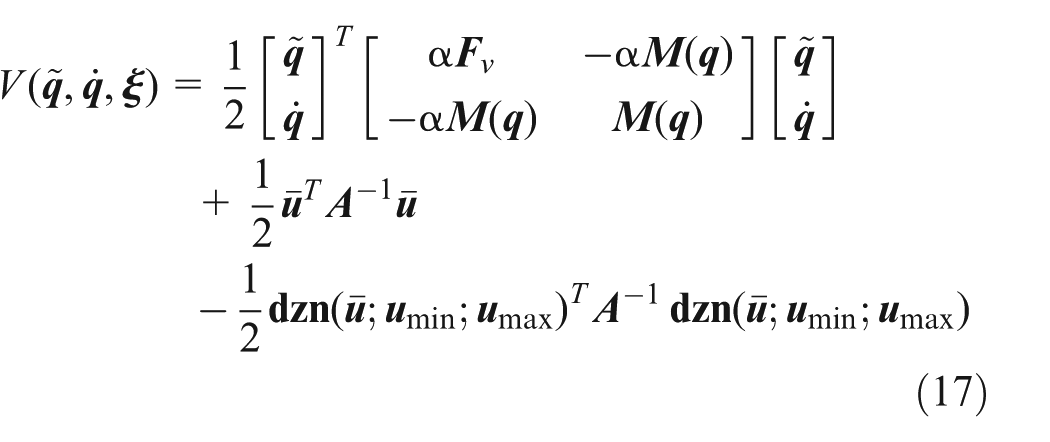
The Lyapunov function candidate proposed by Kanamori15 is used here
where .
Function in equation (17) is continuously differentiable. A proof that function in equation (17) is positive definite is given as follows. First, let us rewrite
where
Function in equation (19) is positive definite because the parameter α satisfies the condition
which is part of the tuning rule (12). Besides, note that
When , it follows
This means that if , the function is strictly positive.
Due to conditions (21) and (22) and equation (23), it follows that and will be fulfilled simultaneously only when . Otherwise, or or both will be positive. Therefore, is positive definite.
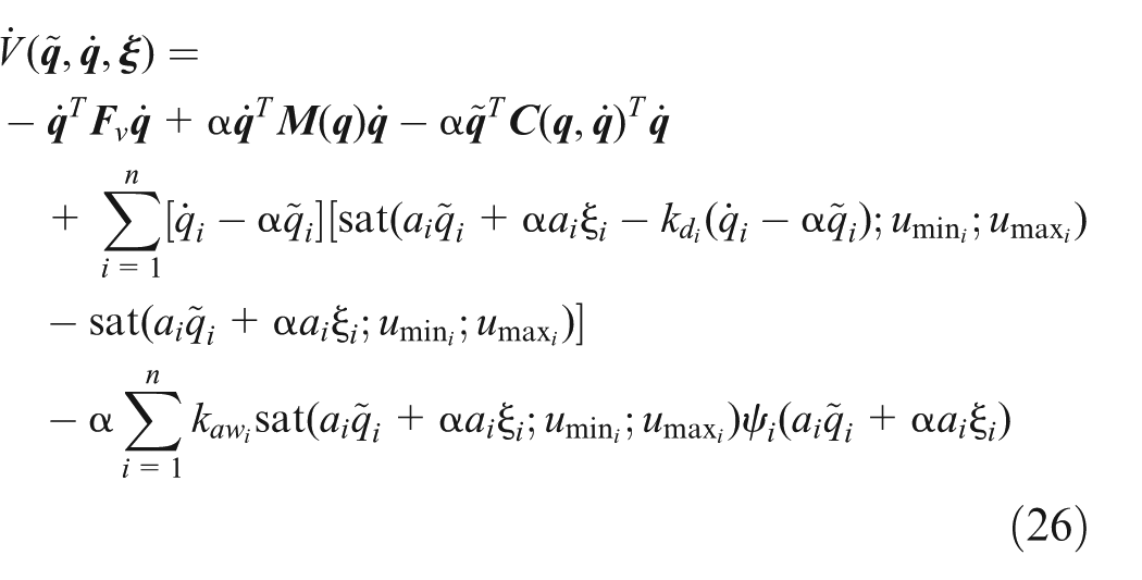
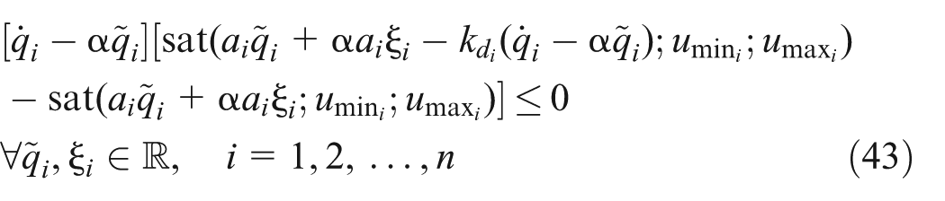
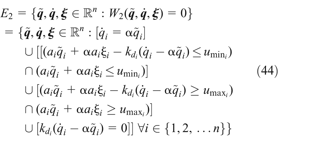
In the following, the local negative definiteness of function in equation (26) is shown. Besides, we present discussions on the sets where , , and are null.
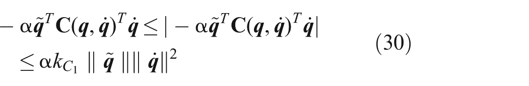
Using Property 3, the term in in equation (27) is upper bounded as follows
which ensures the right-hand side of condition (34) to be positive. Note that condition (35) is part of the tuning rule (12). Therefore, the function in equation (27) satisfies
with γ in condition (34), that is, is a locally negative semi-definite function.
The set of values of that satisfy (36) and make is
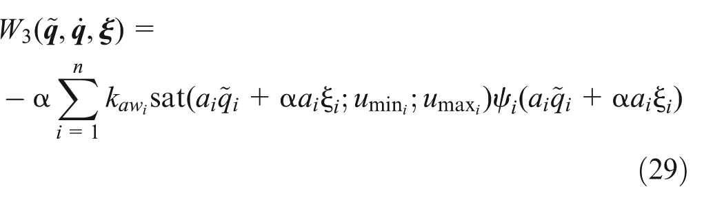
Function in equation (28) is globally negative semi-definite as follows
The origin 0 is the unique point that satisfies set (49).
The negative definiteness of function is assured locally in domain S in equation (48). In agreement to Lyapunov’s direct method stated in Vidyasagar,25 the origin of the state space of equation (16) is locally asymptotically stable (because in equation (17) is a globally positive definite function by condition (21) and in equation (26) is a locally negative definite function by condition (35)). Therefore, the control objective (9) is locally satisfied.
Conditions (21) and (35) are combined to obtain the tuning rule (12) so that with control scheme in equations (10) and (11) the regulation control objective (9) is satisfied.
Actuator protection
Among the controller parameters, only the scalar parameter α must be carefully tuned according to rule (12), which is independent of the saturation levels and . This means that the stability of the origin of the state space of closed-loop system does not rely on the saturation levels of actuators.
According to actuator manufacturers, such as electrical motors, actual physical actuators can operate safely within prescribed torque saturation levels. In order to protect the actuators from damage, their inputs ui should be within the prescribed actuator torque capability. This leads to the following approach to safely control the actuator–robot system.
A remarkable feature of the proposed control law in equations (10) and (11) is that the levels of saturation of the actuators are not required to tune the controller en equations (10) and (11). Given that it is only required that and , an “artificial” hard saturation can be added by programming to protect the actuators (see Figure 6), while the stability of the origin of the state space of the closed-loop system is kept asymptotical.
Addition of an “artificial” hard saturation to protect the actuators.
The “artificial” hard saturation is defined as follows
with and defined as in Proposed control scheme section and
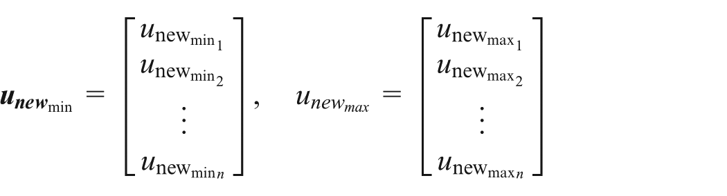
where and are the user-defined saturation levels for the “artificial” hard saturation.
In order to protect the actuators, these artificial saturation levels must be chosen in agreement with
and
which will prevent actuator i to work in the limits of its capacity.
Figure 7 shows a diagram of the closed-loop system with “artificial” hard saturation proposed in (50) and (51). The input u to the “artificial” hard saturation is the output u of the proposed controller in (10) and (11) and the output of the “artificial” hard saturation is the input to the actuator model (3).
Closed-loop system with “artificial” hard saturation and actuator. The block “artificial saturation” is represented by equations (50) and (51). The reason for adding the artificial hard saturation is to protect the actuators.
Combination of the actuator model in equation (3) and the “artificial” saturation in equation (50) leads to
where
Figure 8 shows a diagram of the closed-loop system with “artificial” hard saturation + actuator resulting in equation (54).
Closed-loop system with “artificial” hard saturation + actuator.
The closed-loop system block diagram depicted in Figure 8 is useful for analysis purposes; it has the same structure that system (16), so the same analysis and conclusions from section “Analysis,” apply Mutatis Mutandis.
Therefore, if saturation limits of are within the limits of saturation of the actuators, then the actuators will work safely avoiding the saturation levels of the actuators and regardless of saturation limits in and saturation limits of the actuators, the control objective (9) will be achieved at least locally.
Experimental study
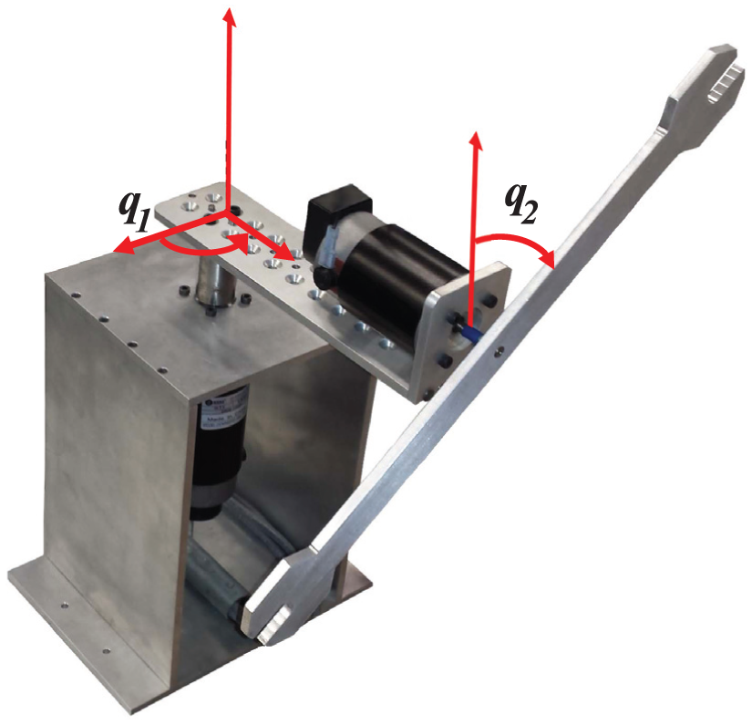
A two DOF direct-drive robot arm located at Instituto Politécnico Nacional-CITEDI was used to illustrate through experiments the theoretical results. A picture of the system is presented in Figure 9.
Two DOF CITEDI I robot arm.
The measurement data are obtained with the data acquisition (DAQ) Sensoray 626 which has input ports for optical encoders, bidirectional input/output digital ports, and analog input/output ports. This DAQ allows interacting with MATLAB/Simulink and performs real-time experiments through Real-Time Windows Target libraries. DC motors from Leadshine Technology. Each motor is powered with an Advanced Motion Controls servo-amplifier. Actuators have optical encoders with a resolution of up to 4000 pulses per revolution.
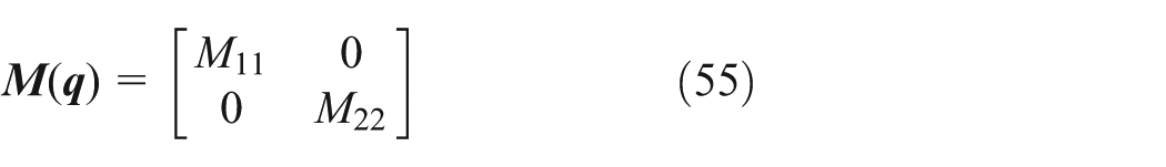
For controller tuning (α parameter in condition (12)) and experimental purposes, the physical parameters of the corresponding robot model (1) are described by
where
The numerical values for , and as well as the saturation limits of the actuators 1 and 2 are listed in Table 1.
Numerical values of parameters of the experimental setup.
Parameter
Value
−1.3455 N m
−0.551 N m
1.3455 N m
0.551 N m
0.0006
0.0031
0.0342
0.0096
The proposed controller in equations (10) and (11) is easily tuned since only one parameter (α in condition (12)) has to be selected via explicit bounds of the robot parameters . Using the values in Table 1, the inequality (12) becomes
For the experiments α is chosen as
Then, inequality (34) becomes
The user-defined functions used in controller presented in equations (10) and (11) were
Since saturation levels of the actuators do not influence the stability, the proposed “artificial” hard saturation was used to protect the actuators. The user-defined saturation levels in condition (52) and in condition (53) were
Using similar conditions, a comparative study of the responses was carried out using the proposed controller in equations (10) and (11), classical linear PID controller (studied in control textbooks26)
To tune the controller described by equations (62) and (63), the α parameter should be carefully chosen so that the following conditions are fulfilled15
Note that the value of α in equation (58) satisfies conditions (64) and (65).
The remaining controller parameters were set to
The three tested controllers, proposed controller (equations (10) and (11)), PID control (equations (60) and (61)), and Kanamori’s law (equations (62) and (63)) have been implemented using the same control gains in equations (58) and (66). The difference of one controller with respect to the others is the form in that the integral action is being computed.
Null initial conditions (joint positions and velocities) were considered in the robot and the constant desired joint position was . So, the initial condition satisfies
Given the restriction of γ in inequality (59), the initial conditions are inside the set S in equation (48).
Experimental results are presented in Figures 10–15. In Figures 10–13, continuous thin gray lines correspond to experimental result using classical linear PID controller in equations (60) and (61), dashed thick brown lines correspond to experimental result using Kanamori’s law in equations (62) and (63), and continuous thick blue lines correspond to experimental result using the proposed controller in equations (10) and (11).
Position of the two DOF robot arm. Continuous thin gray line corresponds to experimental result using classical linear PID controller in equations (60) and (61), dashed thick brown line corresponds to experimental result using Kanamori’s law in equations (62) and (63), and continuous thick blue line corresponds to experimental result using the proposed controller in equations (10) and (11).
Position of the two DOF robot arm. Continuous thin gray line corresponds to experimental result using classical linear PID controller in equations (60) and (61), dashed thick brown line corresponds to experimental result using Kanamori’s law in equations (62) and (63), and continuous thick blue line corresponds to experimental result using the proposed controller in equations (10) and (11).
Output of the “artificial” hard saturation in equations (50) and (51). Continuous thin gray line corresponds to experimental result using classical linear PID controller in equations (60) and (61), dashed thick brown line corresponds to experimental result using Kanamori’s law in equations (62) and (63), and continuous thick blue line corresponds to experimental result using the proposed controller in equations (10) and (11).
Output of the “artificial” hard saturation in equations (50) and (51). Continuous thin gray line corresponds to experimental result using classical linear PID controller in equations (60) and (61), dashed thick brown line corresponds to experimental result using Kanamori’s law in equations (62) and (63), and continuous thick blue line corresponds to experimental result using the proposed controller in equations (10) and (11).
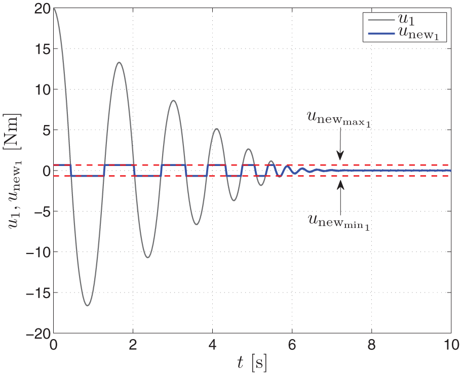
Output of the controller in equations (10) and (11) and output of the “artificial” hard saturation in equations (50) and (51). Continuous thin gray line corresponds to and continuous thick blue line corresponds to .
Output of the controller in equations (10) and (11) and output of the “artificial” hard saturation (50) and (51). Continuous thin gray line corresponds to and continuous thick blue line corresponds to .
Figures 10 and 11 show the actual joint positions and . Note that for the proposed control scheme (equations (10) and (11)) and PID controller in equations (60) and (61), the joint positions and approach and (red dotted lines), respectively. However, the joint positions and obtained by implementing Kanamori’s law (equations (62) and (63)) converge very slowly. The reason for this behavior is the dead-zone function used in equation (63). Numerical simulations for Kanamori’s law (equations (62) and (63)) showed that the actual joint positions and tend to and , respectively, after a long time. Faster convergence could have been obtained for Kanamori’s law selecting smaller gain , which was also verified by numerical simulations.
Note from Figures 10 and 11 that the position responses of the tested schemes (classical PID controller, Kanamori’s law, and the proposed control scheme) are under-damped. What is intended with these results is to allow observing the effect of saturation of the three controllers.
Figures 12 and 13 show the outputs and of the “artificial” hard saturation in equations (50) and (51) (input to the actuator model (3)). The outputs and are kept within the limits of saturation (horizontal red dotted lines).
Figure 14 shows in continuous thin gray line the output of the proposed controller (equations (10) and (11)) and in continuous thick blue line the output of the “artificial” hard saturation (equations (50) and (51)). Figure 15 shows in continuous thin gray line the output of the proposed controller (equations (10) and (11)) and in continuous thick blue line the output of the “artificial” hard saturation (equations (50) and (51)). The outputs and remain within the new saturation limits despite the high values in the controller outputs and .
Results and conclusion
Considering position regulation with torque limitation for robot manipulators of n-DOF having viscous friction but without gravity vector, a family of controllers with easy tuning of its parameters is proposed to ensure the control objective. Considering hard (non differentiable) saturation in the actuators, this family of controllers allows the goal of position control to be achieved in a local sense and can help protect the actuators due to the fact that the stability conditions of the origin of the state space of closed-loop system do not depend on the saturation levels of actuators.
An extensive experimental study in a two DOF robot manipulator was given. The experimental tests allowed comparing the position regulation performance of the classical linear PID controller, Kanamori’s law, and the proposed controller derived from the proposed family of controllers.
Footnotes
Appendix 1
Academic Editor: Yong Tao
Declaration of conflicting interests
The author(s) declared no potential conflicts of interest with respect to the research, authorship, and/or publication of this article.
Funding
The author(s) disclosed receipt of the following financial support for the research, authorship, and/or publication of this article: This work was supported by CONACyT (grant numbers 166654 and 176587).
References
1.
GaleaniSTarbouriechSTurnerM. A tutorial on modern anti-windup design. Eur J Contr2009; 15: 418–440.
2.
Moreno-ValenzuelaJCampaR.Two classes of velocity regulators for input-saturated motor drivers. IEEE Trans Indus Electr2009; 56: 2190–2202.
3.
SuarezRAlvarezJAlvarezJ.Linear systems with single saturated input: stability analysis. In: Proceedings of the 30th IEEE conference on decision and control, Brighton, England, 11–13 December 1991, pp.223–228. New York: IEEE.
4.
KothareMVCampoPJMorariM.A unified framework for the study of anti-windup designs. Automatica1994; 30: 1869–1863.
5.
KothareMVMorariM.Multiplier theory for stability analysis of anti-windup control systems. Automatica1999; 35: 917–928.
6.
TarbouriechSGarciaGGomes da SilvaJMJr. Stability and stabilization of linear systems with saturating actuators. London: Springer-Verlag, 2011.
7.
RobinettRDParkerGGSchaubH. Lyapunov optimal saturated control for nonlinear systems. J Guidance Contr Dyn1997; 20: 1083–1088.
8.
Gomes da SilvaJMJrOliveiraMZCoutinhoD. Static anti-windup design for a class of nonlinear systems. Int J Robust Nonlinear Contr2012; 24: 793–810.
9.
KellyRSantibañezVBerghuisH.Point-to-point robot control under actuator constraints. Contr Eng Pract1997; 5: 1555–1562.
10.
GorezR.Globally stable PID-like control of mechanical systems. Syst Contr Lett1999; 38: 61–72.
11.
ZergerogluEDixonWBehalA. Adaptive set-point control of robotic manipulators with amplitude-limited control inputs. Robotica2000; 18: 171–181.
12.
DixonW.Adaptive regulation of amplitude limited robot manipulators with uncertain kinematics and dynamics. IEEE Trans Automat Contr2007; 52: 488–493.
13.
Álvarez-RamírezJKellyRCervantesI.Semiglobal stability of saturated linear PID control for robot manipulators. Automatica2003; 39: 989–995.
14.
MorabitoFTeelARZaccarianL.Nonlinear antiwindup applied to Euler–Lagrange Systems. IEEE Trans Robot Automat2004; 20: 526–537.
15.
KanamoriM. Static anti-windup controller design for planar 2DOF robot manipulators with actuator saturation. In: Proceedings of the 2009 IEEE international conference on robotics and automation, Kobe, Japan, 12–17 May 2009, pp.3314–3319. New York: IEEE.
16.
SantibáñezVCamarilloKMoreno-ValenzuelaJ. A practical PID regulator with bounded torques for robot manipulators. Int J Contr Automat Syst2010; 8: 544–555.
17.
YokoyamaMKimGNTsuchiyaM.Integral sliding mode control with anti-windup compensation and its application to a power assist system. J Vib Contr2010; 16: 503–512.
18.
SuYMüllerPCZhengC.Global asymptotic saturated PID control for robot manipulators. IEEE Trans Contr Syst Tech2010; 18: 1280–1288.
19.
IzadbakhshAFatehMM.Real-time robust adaptive control of robots subjected to actuator voltage constraint. Nonlinear Dyn2014; 78: 1999–2014.
20.
SuYSweversJ.Finite-time tracking control for robot manipulators with actuator saturation. Robot Compu Integr Manuf2014; 30: 91–98.
21.
TianHSuY.A repetitive learning method based on sliding mode for robot control with actuator saturation. J Dyn Syst Measure Contr2015; 137: 064505.
22.
SciaviccoLSicilianoB.Modelling and control of robot manipulators. 2nd ed.London: Springer-Verlag, 2000.
23.
KellyRSantibañezVLoríaA.Control of robot manipulators in joint space. London: Springer-Verlag, 2005.
24.
SpongMWHutchinsonSVidyasagarM.Robot modelling and control. Hoboken, NJ: John Wiley & Sons, 2005.
25.
VidyasagarM.Nonlinear systems analysis. 2nd ed.Englewood Cliffs, NJ: Prentice Hall, 1993.
26.
OgataK.Modern control engineering. 5th ed.Englewood Cliffs, NJ: Prentice Hall, 2010.