Sage Journals: Discover world-class research

Abstract

Long-term traffic forecasting has become a basic and critical work in the research on road traffic congestion. It plays an important role in alleviating road traffic congestion and improving traffic management quality. According to the problem that long-term traffic forecasting is short of systematic and effective methods, a long-term traffic situation forecasting model is proposed in this article based on functional nonparametric regression. In the functional nonparametric regression framework, autocorrelation analysis (ACF) is introduced to analyze the autocorrelation coefficient of traffic flow for selecting the state vector, and the functional principal component analysis is also used as distance function for computing proximities between different traffic flow time series. The experiments based on the traffic flow data in Beijing expressway prove that the functional nonparametric regression model outperforms forecast methods in accuracy and effectiveness.

Keywords

Long-term forecasting traffic situation functional nonparametric regression autocorrelation analysis

Introduction

With the rapid urban development and gradually increase in the number of vehicles, traffic congestion has been heavily fixed eyes on. Numerous methods are used to alleviate the problem of congestion. Nowadays, advanced traffic management system (ATMS), advanced traffic information system (ATIS), dynamic route guidance system (DRGS), and other intelligent transportation systems are being applied more widely. Accurate and reliable traffic forecasting, as the basic requirement and key technology of these systems, has also attracted more and more attention. Research on traffic flow forecasting has important theoretical significance and application value.

Traffic forecasting is to speculate the traffic state in the future by analyzing traffic flow data. According to the forecast period, it can be divided into short-term forecasting and long-term forecasting.^1,2 The former refers to the forecast period is short, usually less than 30 min, while the latter means that the forecast period is longer, such as a day, a week, or even longer.

In the early time, forecast methods mainly included time series models, exponential smoothing model, Kalman filter model, and so on.^3,4 With the deepening of the work, some new methods were applied to traffic forecasting, such as nonparametric regression, neural network, support vector machine, wavelet analysis, and others.^5–12

Vlahogianni et al.¹³ briefly discussed the existing research since the early 1980s and then offered information on 10 areas where they believed that the technological and analytical challenges lie for the next generation of short-term forecasting research. Haworth and Cheng¹⁴ employed a nonparametric spatio-temporal kernel regression model to forecast the future values of road links in central London. The model used spatial neighborhood information under the assumption of data that is missing not at random due to sensor failure. Dong et al.¹⁵ divided traffic state into six modes according to the level of service. On the basis of Autoregressive Integrated Moving Average model (ARIMA), the time-delay error in the ARIMA was adjusted dynamically using a dynamic correction function. The analysis showed that the multimode traffic volume prediction model provides a better performance than ARIMA model. Sun et al.¹⁶ provided a multimode maximum entropy model (MME) to deal with regional traffic state. In the research, the different state behaviors were divided into 14 traffic modes defined by average speed according to the date-time division. The experiments proved that the MME models outperform the already existing model in both effectiveness and robustness. Classifying traffic condition states as congestion and non-congestion, Dong et al.¹⁷ proposed multivariate state space models for network flow rate and time mean speed predictions. The study suggested the Non-congestion State Space model (NSS) is better for flow rate prediction under non-congestion conditions, and the Congestion State Space model (CSS) is better for time mean speed prediction under congestion conditions. Min and Wynter¹⁸ provided an extended time-series–based approach of speed and volume predictions over 5-min intervals for up to 1 h in advance. Tchrakian et al.¹⁹ formulated and demonstrated the use of a technique based on spectral analysis for within-day real-time traffic flow forecasting, and the choice of step, historical data, and forecasting horizon were discussed with numerical results. Many prediction methods lead to inefficient predictions when current or future time series data exhibit fluctuations or abruptly change. In order to deal with this problem, Chang et al.²⁰ introduced a dynamic multi-interval traffic volume prediction model based on the k-nearest neighbor nonparametric regression (KNNNPR). Qiao et al.²¹ used traffic and weather data from multiple data sources to develop an integrated model that could predict travel times under various weather conditions, especially severe weather conditions. Considering traffic flow data reveals seasonal trend. Hong²² presented a traffic flow forecasting model that combines the seasonal support vector regression model with chaotic immune algorithm (SSVRCIA), to forecast inter-urban traffic flow. Chrobok et al.²³ organized the historical traffic data into four basic classes and a matching process that assigns these sets into their class automatically is proposed and then proposed two models for short-term forecast: the constant and the linear model. The results show that the constant model provides a good prediction for short horizons whereas the heuristics is better for longer times. In general, throughout the literatures mentioned above, it is true that many researchers have paid attention to traffic forecasting, and many fine prediction methodologies have been reported. Most of the references are limited to focus on short-term traffic forecasting (over 5-min intervals for up to 1 h in advance), especially focus on improving the forecasting accuracy and developing methodologies that can be used to model traffic characteristics such as volume, density, and speed, or travel times, but a little focus on long-term forecasting and lack in the study of the long-term trend of traffic flow. Furthermore, it is turned out that the prediction methodologies work very well for short-term traffic forecasting, in particular accuracy, effectiveness, and stability; however, it is be worth further discussing whether they are suitable for long-term forecasting. Finally, accurate long-term traffic forecasting plays a positive role in improving the quality of traffic management and service. It can provide useful reference not only for increasing efficiency of the limited traffic management resource, such as making reasonable arrangements for police resource upon the long-term forecasting results, but also for helping travelers make plans for a long term in advance to avoid congestion. Hence, long-term traffic forecasting can be considered as the key to achieve traffic management from passive adaptation to active response.

For these reasons, and with the goal of enabling a method to predict the traffic situation in a long term, this work proposes a functional nonparametric regression (FNR) model to predict urban expressway traffic situation over a long term in advance. In the FNR framework, the nonparametric kernel regression is applied to forecast Beijing freeway traffic flow, in which the state vector is selected by analyzing the autocorrelation coefficient of traffic flow. In addition, the application of functional principal component analysis (PCA) to deal with seasonal trend of traffic flow have been used as distance function for computing proximities between different traffic flow time series. The article is structured as follows: the importance of long-term traffic forecasting is emphasized in section “Introduction.” In section “Model,” a mathematical description and the modeling process of the FNR model is given. In section “Case study,” the model has been tested in practice on a Beijing expressway section and the results are analyzed in detail. Finally, we make some conclusions with discussions on future directions in section “Conclusion.”

Model

Functional data analysis (FDA) is a branch of statistics that analyzes data providing information about curves, surfaces, or any other mathematical object. Models and methods for FDA may resemble those for conventional multivariate data, including linear and nonlinear regression models, PCA, and many others.

In order to analyze data with complex structures, the FNR model combines nonparametric regression and FDA, and in such a way that the prediction problem of time series turns to be a standard regression problem.

Traffic is a continuous time stochastic process, time series of traffic flow will be considered as discrete time realizations of a continuous time stochastic process. Since people travel with regularity, traffic flow is a seasonal process. The traffic flow curve of each period can be denoted as equation (1)

X_{i} = {(x_{i} (1), …, x_{i} (J))}^{T}, i = 1, …, n

(1)

where $x_{i} (t)$ is the value at the time t in the ith period, and seasonal length can be a day, a week, a month, a year, and so on. For simplicity, the following property for the process X is assumed as follows

x_{i} (t) | \overset{d}{=} x_{i - 1} (t)

(2)

Equation (2) states that the probability distribution of a future value of the process given only depends on the time series of the last period. That is, the estimation of $x_{i}$ depends on $x_{i - 1}$ .

According to the basic idea for forecasting above, this article uses historical data for forecasting traffic flow in the future based on nonparametric regression method; generally, it can be expressed as follows

Y = g (X) + ε

(3)

where $E [ε | X = x] = 0, Var [ε | X = x] = σ^{2}$ .

Nonparametric regression method is to use the given X in the observation $(X, Y)$ to estimate the value of Y without any restriction in the form of $g (X)$ , so there is no need to establish a precise mathematical model and it fits for nonlinear and time-varying systems.

In the FNR model, the estimation of $g (X)$ using kernel regression method is given by equation (4)

g_{n} (x) = \sum_{i = 1}^{n} W_{i} (x, x_{i}) Y_{i}

(4)

where Y is one-dimensional observation vector and X is m-dimensional independent variable. A N-W type estimator is defined by equation (5)

W_{i} (x, x_{i}) = \frac{K (d (x, x_{i}) / h)}{\sum_{j = 1}^{n} K (d (x, x_{j}) / h)}

(5)

where K is the kernel function, d is the distance function, and h is the bandwidth.

On the basis of equation (2), assuming that observation $(X_{i}, Y_{i}) = (χ_{i - 1}, x_{i}), i = 1, \dots, n$ in equation (4)

x_{i} (t) = g (χ_{i - 1} (t)) + ε, i = 1, \dots, n

(6)

Equation (6) states that the value of the time series $x_{i}$ at time t is an unknown nonparametric function of the last time series $χ_{i - 1}$ at time t plus some error term. Thus, $\hat{g} (χ_{n} (t))$ gives a functional forecast for $x_{n + 1} (t)$ .

Therefore, based on nonparametric regression and N-W type estimator, the long-term traffic forecasting model can be expressed by $x_{n + 1} (t) = \hat{g} (χ_{n} (t)) + ε$ , and then substituting it into equations (4) and (5), we obtain equation (7)

\begin{matrix} x_{n + 1} (t) = \hat{g} (χ_{n} (t)) = \sum_{i = 1}^{n - 1} w_{h} (χ_{n} (t), χ_{i} (t)) x_{i + 1} (t)) \\ = \frac{K (d (χ_{n} (t), χ_{i} (t)) / h)}{\sum_{j = 1}^{n - 1} K (d (χ_{n} (t), χ_{j} (t)) / h)} x_{i + 1} (t) \end{matrix}

(7)

where $\hat{g} (χ_{n})$ is the estimation of $g (x)$ , $x_{n + 1} (t)$ is the predicted value at time t in the (n + 1)th period, $χ_{n} (t)$ is the state vector of the FNR model at time t, and $χ_{i}$ is the historical data in the ith period.

To forecast the traffic flow data, many principal factors, such as the state vector, distance function, kernel function, in the FNR model are important. Finally, the framework and process of the FNR model is represented in Figure 1:

Choose the state vector χ using autocorrelation analysis;

Compute distance function d by the functional PCA;

Select the kernel function K;

Feed into equation (7) to obtain the forecasted values.

Figure 1.

Framework and process of the FNR model.

Choice of state vector

The state vector $χ_{n} (t)$ of the FNR model at time t in equation (6) can be selected using autocorrelation analysis. Autocorrelation analysis describes the correlation degree between two times i, j of time series X, which is in the range of [−1, 1]. The random time series with a total of J observations is divided into J − 1 pairs, that is, $(x_{1}, x_{2}), (x_{2}, x_{3}), (x_{3}, x_{4}), \dots, (x_{J - 1}, x_{J})$ , and then the first-order coefficient of autocorrelation (ACF) is defined by equation (8)²⁴

\begin{matrix} ρ_{1} = \frac{\sum_{i = 1}^{J - 1} (x_{i} - \bar{x_{i}}) (x_{i + 1} - \bar{x_{i + 1}})}{\sqrt{\sum_{i = 1}^{J - 1} {(x_{i} - \bar{x_{i}})}^{2} \sum_{i = 1}^{J - 1} {(x_{i + 1} - \bar{x_{i + 1}})}^{2}}} \\ = \frac{cov (x_{i}, x_{i + 1})}{\sqrt{σ_{x_{i}}^{2}} \sqrt{σ_{x_{i + 1}}^{2}}} \end{matrix}

(8)

In the same way, the time series divided into $J - k$ pairs, the k-order coefficient of autocorrelation is defined as follows

\begin{matrix} ρ_{k} = \frac{\sum_{i = 1}^{J - k} (x_{i} - \bar{x_{i}}) (x_{i + k} - \bar{x_{i + k}})}{\sqrt{\sum_{i = 1}^{J - k} {(x_{i} - \bar{x_{i}})}^{2} \sum_{i = 1}^{J - k} {(x_{i + k} - \bar{x_{i + k}})}^{2}}} \\ = \frac{cov (x_{i}, x_{i + k})}{\sqrt{σ_{x_{i}}^{2}} \sqrt{σ_{x_{i + k}}^{2}}} \end{matrix}

(9)

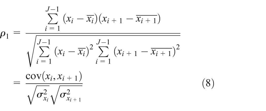
For stationary time series whose expectation is a constant, its observations fluctuate around the expectation; therefore, the variance is also a constant and the k-order autocorrelation coefficient can be expressed as follows

ρ_{k} = \frac{cov (x_{i}, x_{i + k})}{\sqrt{σ_{x_{i}}^{2}} \sqrt{σ_{x_{i + k}}^{2}}} = \frac{cov (x_{i}, x_{i + k})}{σ^{2}}

(10)

In accordance with the theory of autocorrelation analysis, when autocorrelation coefficient is in the range of $[- 1.96 / \sqrt{J}, 1.96 / \sqrt{J}]$ , it can be said that there is no significant difference with 0 (i.e. the correlation degree between the observations is very weak). For example, as can be seen in Figure 2, the first-order and second-order autocorrelation coefficients are not in the range above, that is, $x_{i}$ has greater correlation degree with the observations: $x_{i - 2}$ , $x_{i - 1}$ , $x_{i + 1}$ , $x_{i + 2}$ , and then, the observations above can be used as the state vector to forecast.

Figure 2.

Result of autocorrelation analysis as an example.

Distance function computing

In many multivariate situations, the PCA is considered as a useful tool for displaying data in a reduced dimensional space. More recently, the PCA methods were extended to FDA.^25–27 Here, the functional PCA is used as distance function for computing proximities between different traffic flow curves.

As long as $E \int x^{2} (t) dt$ is finite, the functional PCA allows us to obtain the following expansion

x (t) = \sum_{k = 1}^{q} (\int x (t) ξ_{k} (t) dt) ξ_{k} (t)

(11)

$ξ_{k} (t)$ being orthonormal eigenfunctions of the covariance operator associated with the eigenvalues $λ_{1} \geq λ_{2} \geq \dots \geq λ_{q}$

Γ χ (s, t) = E (χ (s) χ (t))

(12)

Now, equation (11) makes the equation

\sum {‖ χ (t) - \hat{χ} (t) ‖}^{2} = \sum \int {[χ (t) - \hat{χ} (t)]}^{2} dt

(13)

minimum, at that time $\hat{χ} (t)$ will be the optimal estimated value of $χ (t)$ . Thus, a parameterized class of semi-norms from the classical $L^{2}$ norm can be defined by the following way

‖ x ‖_{q}^{PCA} = \sqrt{{\int ({\hat{χ}}^{(q)} (t))}^{2} dt} = \sqrt{\sum_{k = 1}^{q} {(\int x (t) ξ_{k} (t) dt)}^{2}}

(14)

d_{q}^{PCA} (χ_{i}, χ) = \sqrt{\sum_{k = 1}^{q} {(\int [χ_{i} (t) - χ (t)] ξ_{k} (t) dt)}^{2}}

(15)

Note that in practice, we can only observe a discretized version

{X_{i} = {(x_{i} (1), \dots, x_{i} (J))}^{T}}_{i = 1, \dots, n}

(16)

Therefore, the integral can be approximated as follows

\int [χ_{i} (t) - χ (t)] ξ_{k} (t) dt \approx \sum_{j = 1}^{J} w_{j} (χ_{i} (j) - χ (j)) ξ_{k} (j)

(17)

where $w_{1}, \dots, w_{J}$ are quadrature weights which define using a standard choice $w_{j} = t_{j} - t_{j - 1}$ . There are two discretized curves $x_{i}$ and $x'_{i}$ , and the proximities between curves can be approximated as follows

d_{q}^{PCA} (x_{i}, {x'}_{i}) = \sqrt{\sum_{k = 1}^{q} {(\sum_{j = 1}^{J} w_{j} (x_{i} (j) - {x'}_{i} (j)) {[ξ_{k}]}_{j})}^{2}}

(18)

where $ξ_{1}, ξ_{2}, \dots$ are the W-orthonormal eigenvectors of the covariance matrix $(W = diag (w_{1}, \dots, w_{J}))$ associated with the eigenvalues $λ_{1} \geq λ_{2} \geq \dots \geq λ_{q}$

Γ^{J} W = 1 / J \sum_{i = 1}^{J} x_{i}^{T} x_{i} W

(19)

In summary, the parameterized class of semi-norms has a widely application in computing proximities using the functional PCA. Its biggest advantage is that it will be still applicable when the curves are rough relatively. Of course, it also has some defects, that is, each the observations must be in the same time every period, otherwise it will not be able to use the functional PCA.

Kernel function selecting

There are many kernel functions, such as Boxcar kernel, Gaussian kernel, Triangle kernel, and Epanechnikov kernel.²⁸ The Epanechnikov kernel is selected in this model:

Boxcar kernel: $K (x) = 1 / 2 I_{[- 1, 1]} (x)$ ;

Gaussian kernel: $K (x) = 1 / \sqrt{2 π} e^{- x^{2} / 2}$ ;

Triangle kernel: $K (x) = (1 - | x |) I_{[- 1, 1]} (x)$ ;

Epanechnikov kernel: $K (x) = 3 / 4 (1 - x^{2}) I_{[- 1, 1]} (x)$ .

Case study

Experiment scenario and data set

Since people travel with regularity, the traffic flow data with certain rules, there are four different scenarios in 1 week to characterize the rules:

Monday: which is the first day of a week with a high demand, where traffic is large during morning peak and increases significantly; evening peak tends to normal as little difference as usual;

Tuesday to Thursday: which is workday, where traffic is significantly reduced compared to Monday during morning peak and then traffic tends to be basically normal;

Friday: which is the last workday of a week, where traffic is relatively similar to that of the previous day during morning peak, but dramatic increase in evening peak which come too late to go early;

Saturday and Sunday: which is the rest day of a week, where the traffic is small with basically relatively balanced all day.

The FNR model is applied to the four different scenarios (Monday, Wednesday, Friday, and Saturday) for 1-week ahead and 1-day ahead traffic flow forecasting in this work, so the seasonal length of traffic flow defined in equation (1) is 1 week and 1 day, respectively, in the case study.

As mentioned with reference to Figure 3, the target is an expressway section called M1 from Madian Qiao to Anhua Qiao on the inner loop of North 3rd Ring Road Middle in Beijing. Traffic flow data analyzed in this article are collected from the Expressway Traffic Information Detection System in Beijing and obtained daily from the microwave detectors on the expressway. For the survey data sets, the modeling and forecasting are performed on traffic flow data aggregated at 10 min discrete time intervals. Note that $J = 144$ in equation (1). In this research, the traffic flow data are split into two independent samples: the historical data and the test data. The historical data and test data are explained as follows.

Figure 3.

Beijing expressway section M1 location.

One-week ahead forecasting

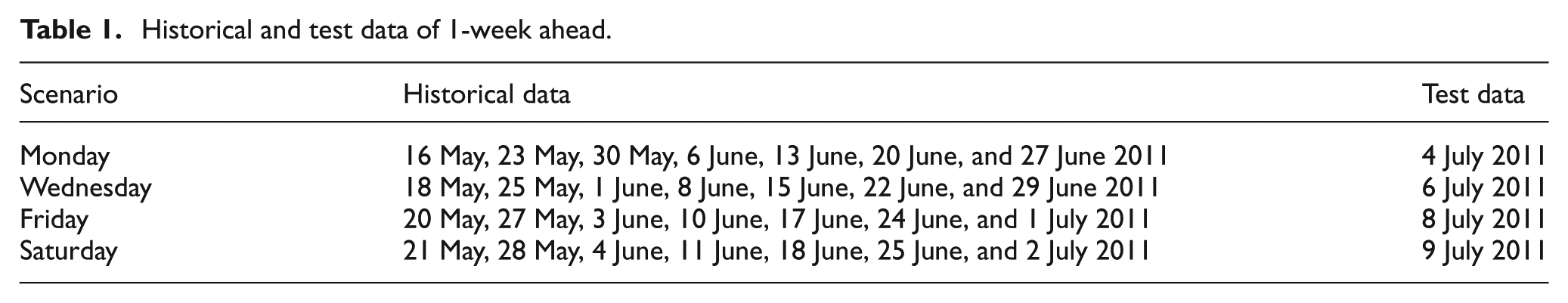
As listed in Table 1, the data between 16 May 2011 and 10 July 2011 (a total of 8 weeks) are split into two parts. The first 7 weeks data of the scenarios (Monday, Wednesday, Friday, and Saturday) are used as historical data, respectively, while the data on 4 July (Monday), 6 July (Wednesday), 8 July (Friday), and 9 July 2011 (Saturday) of the last week as test data to verify the model’s accuracy. Note that $n = 7$ in equation (1).

Table 1.

Historical and test data of 1-week ahead.

Scenario	Historical data	Test data
Monday	16 May, 23 May, 30 May, 6 June, 13 June, 20 June, and 27 June 2011	4 July 2011
Wednesday	18 May, 25 May, 1 June, 8 June, 15 June, 22 June, and 29 June 2011	6 July 2011
Friday	20 May, 27 May, 3 June, 10 June, 17 June, 24 June, and 1 July 2011	8 July 2011
Saturday	21 May, 28 May, 4 June, 11 June, 18 June, 25 June, and 2 July 2011	9 July 2011

One-day ahead forecasting

As listed in Table 2, the data between 20 June and 10 July 2011 are split into two parts. The data of 14 days before Monday, Wednesday, Friday, and Saturday are used as historical data, respectively, while the data on 4 July (Monday), 6 July (Wednesday), 8 July (Friday), and 9 July 2011 (Saturday) as test data to verify the model’s accuracy. Note that $n = 14$ in equation (1).

Table 2.

Historical and test data of 1-day ahead.

Scenario	Historical data	Test data
Monday	20 June to 3 July 2011	4 July 2011
Wednesday	22 June to 5 July 2011	6 July 2011
Friday	24 June to 7 July 2011	8 July 2011
Saturday	25 June to 8 July 2011	9 July 2011

Benchmarks and performance measures

In order to verify the accuracy and effectiveness of the FNR model, forecasts obtained by means of the Seasonal ARIMA model, Back Propagation (BP) network, and Least Squares Support Vector Machine (LSSVM) based on the same date sets mentioned above will be used as benchmarks in this case study.

ARIMA is one of the most popular models for forecasting univariate time series data. When seasonal behavior is included in the model, it can be called Seasonal ARIMA model formed as SARIMA (p, d, q) (P, D, Q).^29–32 BP network^33,34 is a kind of multi-layer network with an input layer, one or more hidden layers and one output layer, which can simulate nonlinear input–output relations and become one of the most widely used neural network model for forecasting. LSSVM^35,36 is an extension of the standard support vector machine, and the calculating speed for forecasting is improved by changing the inequality problem into equation problem.

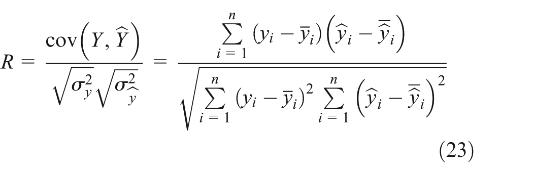
Five different measures of accuracy and effectiveness are used in this research for evaluating the performance of the FNR forecasting model: mean absolute percent error (MAPE), root mean square error (RMSE), consistency index (D),³⁷ correlation coefficient (R), and statistic test (S₁)³⁸ defined by as follows. MAPE is calculated to understand the overall performance of the FNR model; RMSE is useful for understanding the deviation between actual and forecasted values for each forecasting output; D and R are computed to identify the relationships between actual and forecasted values (i.e. the closer the value to 1, the better the performance of the model); and S₁ is a statistic for testing the null hypothesis of no difference in the accuracy of two competing forecasts

MAPE = \frac{1}{n} \sum_{i = 1}^{n} | \frac{y_{i} - {\hat{y}}_{i}}{y_{i}} |

(20)

RMSE = \sqrt{\frac{1}{n} \sum_{i = 1}^{n} {(y_{i} - {\hat{y}}_{i})}^{2}}

(21)

D = 1 - \frac{\sum_{i = 1}^{n} {(y_{i} - {\hat{y}}_{i})}^{2}}{\sum_{i = 1}^{n} {(| y_{i} - \bar{y} | + | {\hat{y}}_{i} - \bar{y} |)}^{2}}

(22)

R = \frac{cov (Y, \hat{Y})}{\sqrt{σ_{y}^{2}} \sqrt{σ_{\hat{y}}^{2}}} = \frac{\sum_{i = 1}^{n} (y_{i} - {\bar{y}}_{i}) ({\hat{y}}_{i} - {\bar{\hat{y}}}_{i})}{\sqrt{\sum_{i = 1}^{n} {(y_{i} - {\bar{y}}_{i})}^{2} \sum_{i = 1}^{n} {({\hat{y}}_{i} - {\bar{\hat{y}}}_{i})}^{2}}}

(23)

where $y_{i}$ is actual values, ${\hat{y}}_{i}$ is forecasted values, $\bar{y}$ is the average of actual values, and ${\bar{\hat{y}}}_{i}$ is the average of forecasted values

S_{1} = \frac{\bar{d}}{\sqrt{\frac{2 π {\hat{f}}_{d} (0)}{n}}} ~ N (0, 1)

(24)

where

d = g (y_{i} - {\hat{y}}_{im}) - g (y_{i} - {\hat{y}}_{in})

(25)

is a loss differential series

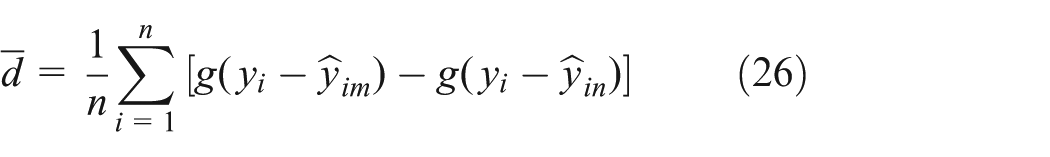
\bar{d} = \frac{1}{n} \sum_{i = 1}^{n} [g (y_{i} - {\hat{y}}_{im}) - g (y_{i} - {\hat{y}}_{in})]

(26)

is the mean loss differential, $y_{i}$ is the actual values, ${\hat{y}}_{im}$ is forecasted values of the mth forecast model

{\hat{f}}_{d} (0) = \frac{1}{2 π} \sum_{τ = - (n - 1)}^{(n - 1)} 1 (\frac{τ}{S (n)}) {\hat{γ}}_{d} (τ)

(27)

is a consistent estimate of the spectral density of the loss differential at frequency zero

{\hat{γ}}_{d} (τ) = \frac{1}{n} \sum_{t = | τ | + 1}^{n} (d_{t} - \bar{d}) (d_{t - | τ |} - \bar{d})

(28)

is the autocovariance of the loss differential at displacement $τ$

1 (\frac{τ}{S (n)}) = {\begin{matrix} 1 & for | \frac{τ}{S (n)} | \leq 1 \\ 0 & otherwise \end{matrix}

(29)

$S (n)$ is the truncation lag.

For the sample, if S₁ is in the range of [−1.96, 1.96], we should accept the null hypothesis that the population mean of the loss differential series is 0, that is, there is equal forecast accuracy for two forecasts.

Results on 1-week ahead forecasting

Upon the traffic flow data from the microwave detectors split into two independent samples, the learning process is initiated to ensure the effectiveness of the original traffic data and consider pruned curves before applying the FNR model to reduce the problem of outlier effect. In this study, as shown in Figure 4, the process of the case study can be described as follows:

Data preprocessing to identify and repair traffic flow fault data (including missing and abnormal data).

Getting the pruned curves of the historical traffic flow curves.

Select the state vector using the autocorrelation coefficient between any two times of the pruned curve.

Get the forecasted values X_n ₊ ₁ with different h by FNR model.

Compute the MAPEs with different h.

Choose the forecasted values when MAPE is the smallest as the final results.

Figure 4.

Process of the case study.

Missing or abnormal data are unavoidable in practice, so it is necessary for data preprocessing to ensure the effectiveness of the original traffic data. In the research, the fault data were removed and repaired by estimating data from values of neighboring detectors or historical data.³⁹ Then, more specifically, the historical traffic flow curves could be pruned in the following way:⁴⁰

Taking the median in $x (t - 2), x (t - 1), x (t), x (t + 1), x (t + 2)$ to form a new smoothing processing $x' (t)$ ;

Taking the median in $x' (t - 1), x' (t), x' (t + 1)$ to form a new smoothing processing $x ″ (t)$ ;

Forming a new smoothing processing $x ‴ (t)$ using the following way

x ‴ (t) = \frac{1}{4} x ″ (t - 1) + \frac{1}{2} x ″ (t) + \frac{1}{4} x ″ (t + 1)

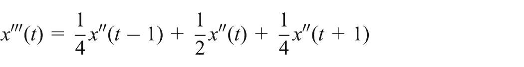
Figure 5 shows the pruned curves from the historical traffic flow data corresponding to the four scenarios.

Figure 5.

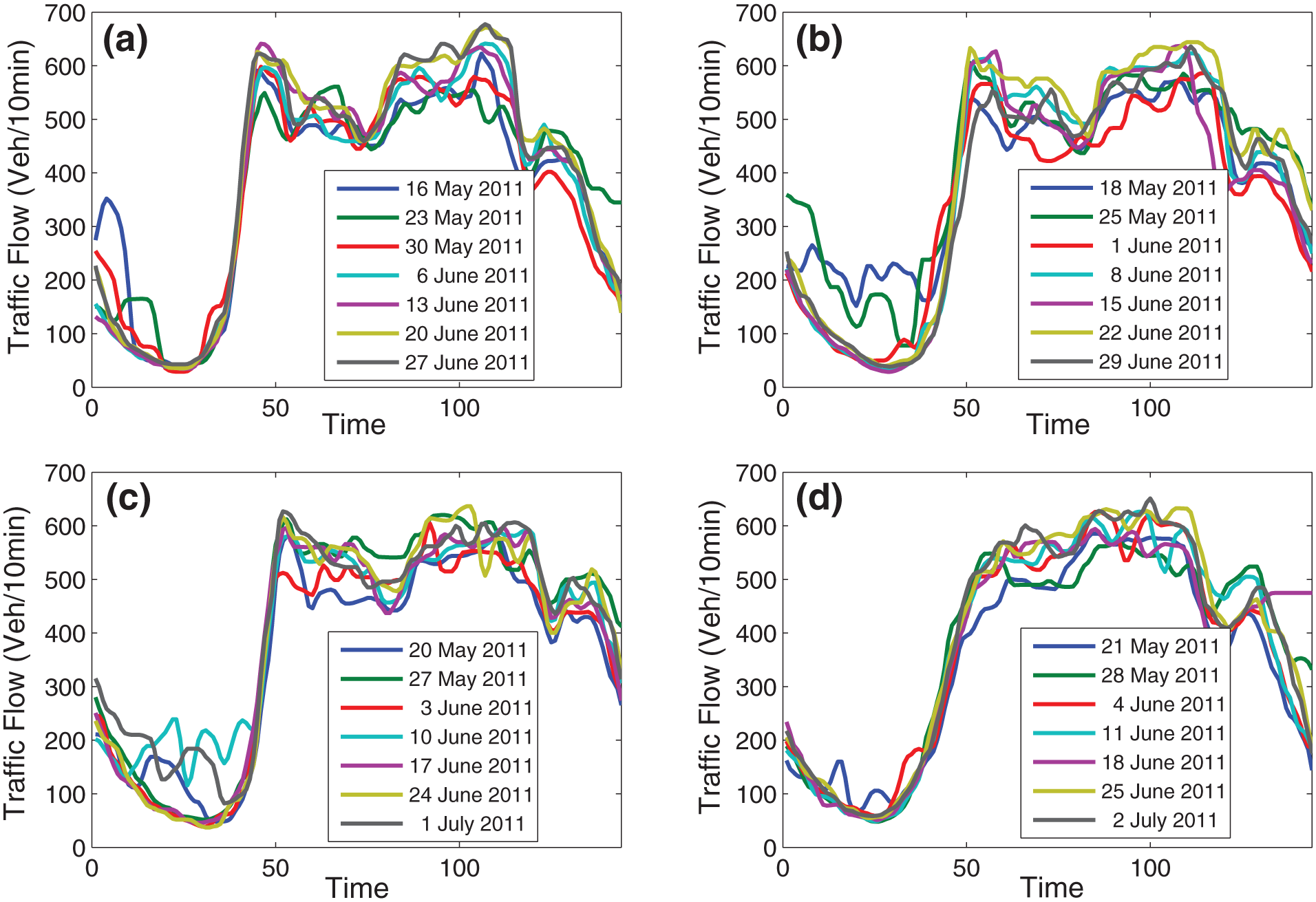
Pruned curves from the historical traffic flow data for 1-week ahead forecasting corresponding to the four scenarios: (a) Monday, (b) Wednesday, (c) Friday, and (d) Saturday.

In the FNR framework, autocorrelation analysis (ACF) is introduced to select the state vector $χ_{n} (t)$ using the autocorrelation coefficient between any two times of the pruned curve. Figure 6 gives the results of traffic flow autocorrelation analysis for the four scenarios.

Figure 6.

Traffic flow autocorrelation coefficient, after first differencing, for the four different scenarios: (a) Monday. The first four autocorrelation coefficients are not within the limit; (b) Wednesday. The first-order coefficient is not within the limit; (c) Friday. The first-order coefficient is not within the limit; and (d) Saturday. The first-order, second-order, and third-order coefficient are not within the limit.

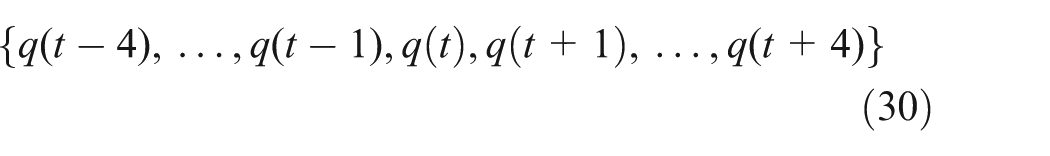
Equations (30)–(33) give the choice of the state vectors for FNR model 1-week ahead forecasting on Monday, Wednesday, Friday, and Saturday, where $q (t)$ is the traffic flow at time t, $Veh / 10 min$ :

Model state vector on Monday as follows

{q (t - 4), \dots, q (t - 1), q (t), q (t + 1), \dots, q (t + 4)}

(30)

Model state vector on Wednesday as follows

{q (t - 1), q (t), q (t + 1)}

(31)

Model state vector on Friday as follows

{q (t - 1), q (t), q (t + 1)}

(32)

Model state vector on Saturday as follows

{q (t - 3), \dots, q (t - 1), q (t), q (t + 1), \dots, q (t + 3)}

(33)

Using the FNR model for forecasting, the bandwidth h is a relevant parameter for the good asymptotic and practical behavior of the model. Here, the optimal bandwidth h could be determined through the performance of MAPE. Figure 7 shows the MAPEs of FNR model 1-week ahead forecasting with different values of h corresponding to the four scenarios. Based on the results, we can choose the optimal bandwidth h as follows: h = 566.2 on Monday, h = 479.4 on Wednesday, h = 424.2 on Friday, and h = 237.4 on Saturday, when the MAPE is the smallest.

Figure 7.

Performance of MAPE for 1-week ahead forecasting varying with the different h: (a) performance of MAPE on Monday, (b) performance of MAPE on Wednesday, (c) performance of MAPE on Friday, and (d) performance of MAPE on Saturday.

In order to obtain the performance of the FNR model in different times, the forecasting accuracy is measured according to two periods: 0:00–24:00 and 6:00–22:00. In addition, SARIMA model, BP network, and LSSVM are used for comparison. Figures 8 –11 display the traffic flow comparisons between actual and 1-week ahead forecasted values of the four scenarios.

Figure 8.

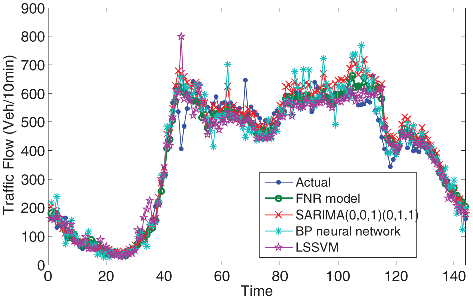
Traffic flow comparisons between actual and 1-week ahead forecasted values on 4 July 2011 (Monday).

Figure 9.

Traffic flow comparisons between actual and 1-week ahead forecasted values on 6 July 2011 (Wednesday).

Figure 10.

Traffic flow comparisons between actual and 1-week ahead forecasted values on 8 July 2011 (Friday).

Figure 11.

Traffic flow comparisons between actual and 1-week ahead forecasted values on 9 July 2011 (Saturday).

Table 3 gives the 1-week ahead forecasting performance (MAPE, RMSE, D, R) comparisons of the FNR model and other models according to two periods: 0:00–24:00 and 6:00–22:00. In general, the results in this table show the good behavior of the FNR model. The FNR model gives slightly better results than the others do. As an example, the FNR model produces a relatively high accuracy of less than 10% error in MAPE. MAPE of the FNR model measured from 0:00 to 24:00 are 9.76% on Monday, 9.32% on Wednesday, 7.99% on Friday, and 7.67% on Saturday, while SARIMA model are 11.12% on Monday, 11.01% on Wednesday, 23.05% on Friday, and 10.59% on Saturday.

Table 3.

Forecasting accuracy comparisons of the FNR model and other models according to the two periods: 0:00–24:00 and 6:00–22:00.

Scenarios	Model	0:00–24:00				6:00–22:00
Scenarios	Model	MAPE	RMSE	D	R	MAPE	RMSE	D	R
4 July 2011 (Monday)	FNR model	9.76%	44.5	0.9882	0.9766	8.18%	52.9	0.9130	0.8346
	SARIMA	11.12%	56.9	0.9821	0.9747	10.33%	68.4	0.8709	0.8214
	BP neural network	14.40%	61.7	0.9780	0.9584	10.26%	71.4	0.8635	0.7626
	LSSVM	12.66%	55.4	0.9809	0.9634	8.81%	64.6	0.8671	0.7527
6 July 2011 (Wednesday)	FNR model	9.32%	38.1	0.9914	0.9849	5.70%	44.8	0.9436	0.9107
	SARIMA	11.01%	51.7	0.9834	0.9822	8.67%	61.4	0.8951	0.9100
	BP neural network	14.17%	51.5	0.9836	0.9750	8.69%	56.7	0.9062	0.8675
	LSSVM	10.37%	48.1	0.9861	0.9778	7.70%	56.1	0.9146	0.8691
8 July 2011 (Friday)	FNR model	7.99%	39.5	0.9903	0.9831	6.53%	46.5	0.9226	0.8751
	SARIMA	23.05%	54.8	0.9806	0.9704	8.10%	54.9	0.9029	0.8215
	BP neural network	14.95%	56.7	0.9813	0.9650	9.44%	64.8	0.8653	0.7624
	LSSVM	14.86%	52.7	0.9822	0.9670	7.43%	60.6	0.8789	0.7833
9 July 2011 (Saturday)	FNR model	7.67%	35.5	0.9920	0.9852	7.14%	42.2	0.9648	0.9401
	SARIMA	10.59%	45.0	0.9876	0.9814	9.23%	52.8	0.9509	0.9250
	BP neural network	11.29%	51.9	0.9824	0.9655	9.20%	56.7	0.9320	0.8774
	LSSVM	13.43%	45.2	0.9865	0.9747	9.09%	49.0	0.9477	0.9145

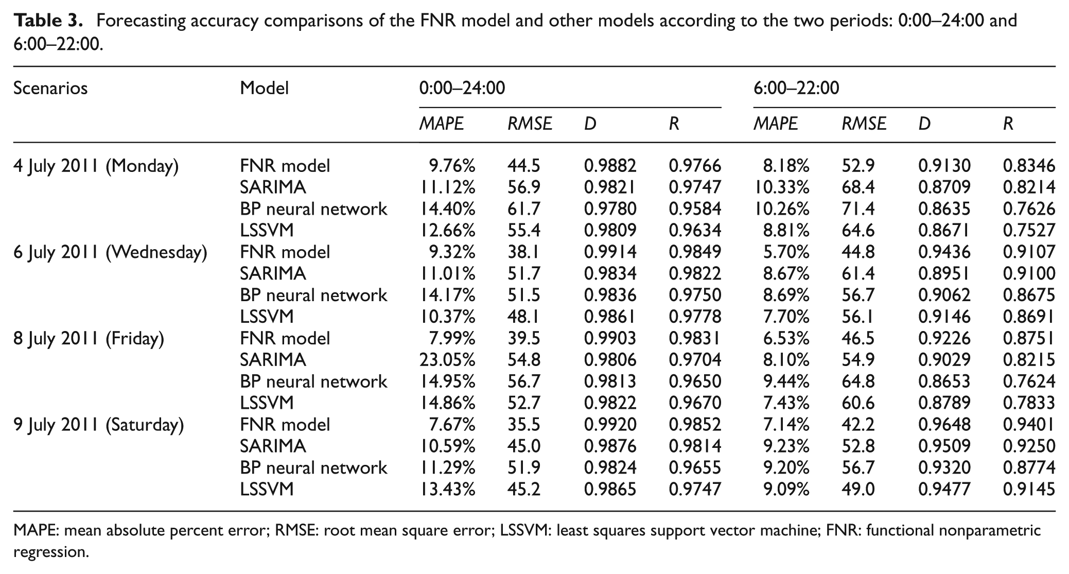
MAPE: mean absolute percent error; RMSE: root mean square error; LSSVM: least squares support vector machine; FNR: functional nonparametric regression.

Table 4 shows the statistic test S₁ of 1-week ahead forecasted values between the FNR model and benchmarks. Since S₁ is not in the range of [−1.96, 1.96], it could be said that there is significantly difference in the forecasting accuracy between FNR model and benchmarks.

Table 4.

Statistic S₁ of 1-week ahead forecasted values between the FNR model and benchmarks according to the two periods: 0:00–24:00 and 6:00–22:00.

Scenarios	Model	0:00–24:00			6:00–22:00
Scenarios	Model	SARIMA	BP neural network	LSSVM	SARIMA	BP neural network	LSSVM
4 July 2011 (Monday)	FNR model	−2.1264	−2.5428	−2.1052	−2.2707	−2.0412	−2.0609
6 July 2011 (Wednesday)		−3.3185	−3.4659	−2.2802	−5.2577	−3.8749	−2.2361
8 July 2011 (Friday)		−2.8799	−3.7373	−2.1477	−2.0488	−2.4097	−2.0499
9 July 2011 (Saturday)		−2.8656	−3.1704	−3.3244	−2.2273	−3.4012	−2.2392

LSSVM: least squares support vector machine; FNR: functional nonparametric regression.

Figure 12 displays a visual comparison of MAPE corresponding to each model for 1-week ahead forecasting. Although the four models exhibit comparable results, the best behavior of the FNR model is also evident from this plot.

Figure 12.

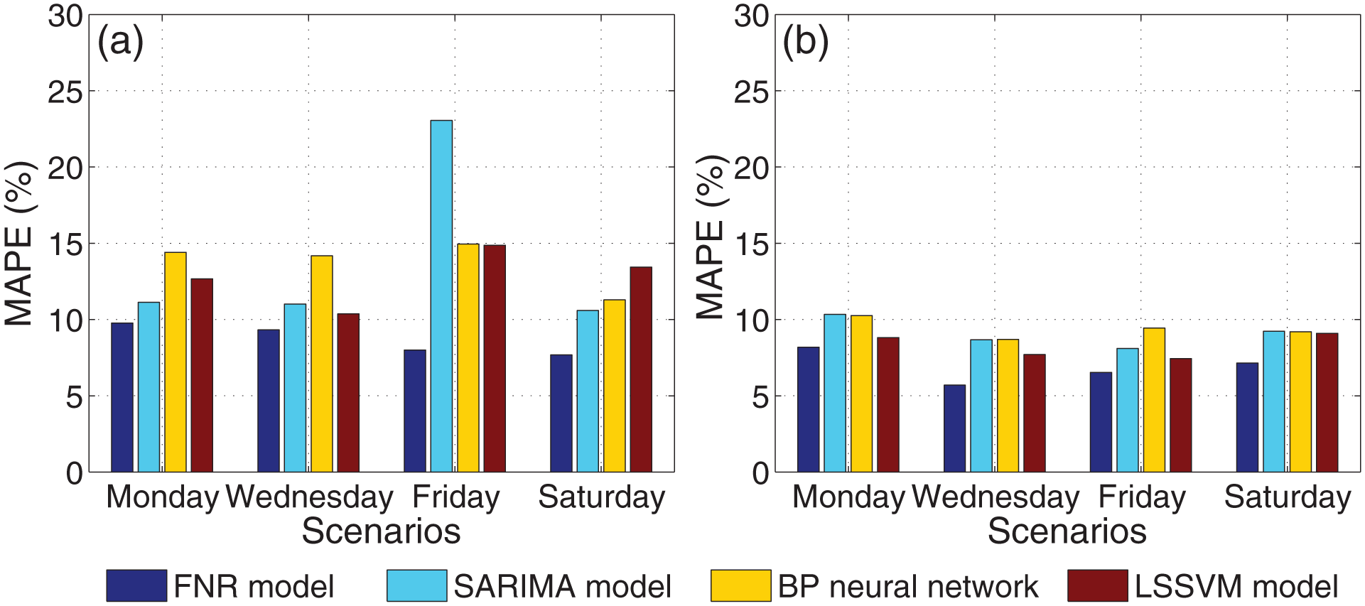
Comparison of MAPE corresponding to each model for 1-week ahead forecasting: (a) measured from 0:00 to 24:00 and (b) measured from 6:00 to 22:00.

Results on 1-day ahead forecasting

In accordance with the process shown in Figure 4, a similar study is conducted in this section for traffic flow 1-day ahead forecasting. In addition, the benchmarks and measures to evaluate the performance of FNR model are also the same as the previous 1-week ahead forecasting.

Figure 13 shows the MAPEs of FNR model 1-day ahead forecasting with different values of h corresponding to the four scenarios. Based on the results, we can choose the optimal bandwidth h as follows: h = 356.3 on Monday, h = 304.3 on Wednesday, h = 388.0 on Friday, and h = 212.6 on Saturday, when the MAPE is the smallest.

Figure 13.

Performance of MAPE for 1-day ahead forecasting varying with the different h: (a) performance of MAPE on Monday, (b) performance of MAPE on Wednesday, (c) performance of MAPE on Friday, and (d) performance of MAPE on Saturday.

As the same as the 1-week ahead forecasting, the forecasting accuracy of 1-day ahead forecasting is also measured according to two periods: 0:00–24:00 and 6:00–22:00, SARIMA model, BP network, and LSSVM are also used for comparison. Figures 14 –17 display the traffic flow comparisons between actual and 1-day ahead forecasted values of the four scenarios. Table 5 gives the 1-day ahead forecasting performance (MAPE, RMSE, D, R) comparisons of the FNR model and other models according to two periods: 0:00–24:00 and 6:00–22:00. Table 6 shows the statistic S₁ of 1-day ahead forecasted values between the FNR model and benchmarks. Finally, Figure 18 displays a comparison of MAPE of the four models for 1-day ahead forecasting.

Figure 14.

Traffic flow comparisons between actual and 1-day ahead forecasted values on 4 July 2011 (Monday).

Figure 15.

Traffic flow comparisons between actual and 1-day ahead forecasted values on 6 July 2011 (Wednesday).

Figure 16.

Traffic flow comparisons between actual and 1-day ahead forecasted values on 8 July 2011 (Friday).

Figure 17.

Traffic flow comparisons between actual and 1-day ahead forecasted values on 9 July 2011 (Saturday).

Table 5.

Forecasting accuracy comparisons of the FNR model and other models according to the two periods: 0:00–24:00 and 6:00–22:00.

Scenarios	Model	0:00–24:00				6:00–22:00
Scenarios	Model	MAPE	RMSE	D	R	MAPE	RMSE	D	R
4 July 2011 (Monday)	FNR model	10.45%	48.0	0.9862	0.9729	8.88%	57.3	0.9058	0.8257
	SARIMA	16.07%	79.1	0.9620	0.9258	13.05%	95.0	0.7878	0.6554
	BP neural network	12.53%	61.2	0.9786	0.9602	10.30%	72.9	0.8551	0.7474
	LSSVM	13.05%	53.8	0.9830	0.9684	9.68%	63.5	0.8833	0.7897
6 July 2011 (Wednesday)	FNR model	8.95%	42.8	0.9893	0.9795	6.31%	50.6	0.9287	0.8686
	SARIMA	11.20%	54.9	0.9815	0.9710	8.90%	66.0	0.8851	0.8599
	BP neural network	12.17%	58.4	0.9794	0.9609	8.39%	66.7	0.8812	0.7809
	LSSVM	10.98%	52.0	0.9844	0.9693	8.22%	62.0	0.9014	0.8149
8 July 2011 (Friday)	FNR model	7.95%	37.8	0.9912	0.9832	6.85%	45.4	0.9338	0.8782
	SARIMA	13.64%	43.4	0.9882	0.9788	7.67%	50.0	0.9320	0.8446
	BP neural network	11.22%	48.3	0.9864	0.9745	8.06%	56.3	0.9109	0.8439
	LSSVM	13.71%	51.9	0.9828	0.9681	9.31%	61.0	0.8856	0.8057
9 July 2011 (Saturday)	FNR model	8.93%	41.4	0.9890	0.9788	8.88%	49.5	0.9445	0.9211
	SARIMA	13.58%	64.9	0.9723	0.9500	13.51%	78.7	0.9382	0.7745
	BP neural network	11.66%	54.1	0.9817	0.9653	11.59%	65.0	0.9111	0.8481
	LSSVM	14.44%	60.8	0.9773	0.9574	12.53%	725.8	0.8743	0.8168

MAPE: mean absolute percent error; RMSE: root mean square error; FNR: functional nonparametric regression; LSSVM: least squares support vector machine.

Table 6.

Statistic S₁ of 1-day ahead forecasted values between the FNR model and benchmarks according to the two periods: 0:00–24:00 and 6:00–22:00.

Scenarios	Model	0:00–24:00			6:00–22:00
Scenarios	Model	SARIMA	BP neural network	LSSVM	SARIMA	BP neural network	LSSVM
4 July 2011 (Monday)	FNR model	−2.0297	−2.121	−2.3008	−2.0345	−1.9983	−2.0443
6 July 2011 (Wednesday)		−2.3229	−2.7569	−2.6689	−2.1376	−2.2815	−2.6118
8 July 2011 (Friday)		−2.8033	−3.4868	−2.4961	−2.0587	−2.2111	−2.0786
9 July 2011 (Saturday)		−2.1438	−2.6447	−2.0378	−2.0618	−2.8459	−2.0653

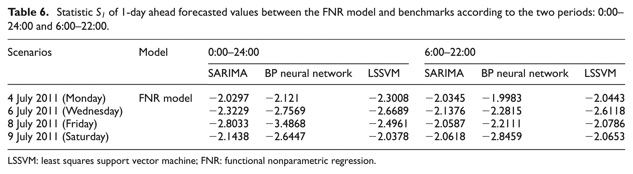
LSSVM: least squares support vector machine; FNR: functional nonparametric regression.

Figure 18.

Comparison of MAPE corresponding to each model for 1-day ahead forecasting: (a) measured from 0:00 to 24:00 and (b) measured from 6:00 to 22:00.

Examining those table and figures above, the following statements could be drawn:

Table 5 gives the 1-day ahead forecasting performance (MAPE, RMSE, D, R) comparisons of the FNR model and other models according to two periods: 0:00–24:00 and 6:00–22:00. It is also clear that the FNR model is a very competitive one for traffic flow long-term forecasting. In this case, the FNR model produces a relatively high accuracy in MAPE. MAPE of the FNR model measured from 0:00 to 24:00 are 10.45% on Monday, 8.95% on Wednesday, 7.95% on Friday, and 8.93% on Saturday, while SARIMA model are 16.07% on Monday, 11.20% on Wednesday, 13.64% on Friday, and 13.58% on Saturday.

Table 6 shows the statistic S₁ of 1-day ahead forecasted values between the FNR model and benchmarks. It is clear that there is difference in the accuracy between FNR model and others.

Figure 18 displays a comparison of MAPE of the four models for 1-day ahead forecasting, and the competitive behavior of FNR model is also clearly seen from this figure.

In summary, the proposed FNR model is generally better than other models in both accuracy and effectiveness and performs well in the 1-week ahead and 1-day ahead forecasting. Complementary, it can be easily applied to other frequency data (e.g. 2 min data, hourly data) whenever they become available.

Conclusion

Long-term traffic forecasting of urban freeway has become a basic and critical work in the research on road traffic congestion. It plays a positive role in improving the quality of traffic management and service. On one hand, it is helpful for increasing efficiency of the limited traffic management resource, especially, making reasonable arrangements for police or other management resource. On the other hand, it can provide useful reference for travelers to make plans for a long term in advance to avoid congestion. The goal of this work is to develop a highly accurate method for traffic situation long-term forecasting. The FNR model is introduced, and that goal is clearly achieved by this effort. The advantages of the FNR framework are as follows:

Temporal features of traffic flow are considered. In the FNR framework, in order to select the state vector of FNR model, the common variation characteristics are analyzed by the autocorrelation coefficient between any two times of traffic flow data.

The differences of long-term change trends are got from the historical traffic flow data by computing proximities based on the functional PCA.

Moreover, the experiments based on the traffic flow data in Beijing expressway show that the FNR model performs better than other models in both accuracy and effectiveness. Complementary, it can be easily applied to other frequency data whenever they become available. All these features make this approach appealing and with plenty of potential for improving. The next steps of this work are to refine the model incorporating spatial features of traffic flow and summarize long-term forecasting of the road network under the FNR model.

Footnotes

Academic Editor: Chin-Lung Chen

Declaration of conflicting interests

The author(s) declared no potential conflicts of interest with respect to the research, authorship, and/or publication of this article.

Funding

The author(s) disclosed receipt of the following financial support for the research, authorship, and/or publication of this article: This work was supported in part by the National Science & Technology Pillar Program (Grant No. 2014BAG 01B02).

References

Smith

Williams

Oswald

RK.

Comparison of parametric and non-parametric models for traffic flow forecasting. Transport Res C: Emer 2002; 10: 303–321.

Dong

CJ.

Theoretical research for short-term traffic flow prediction in multi traffic states on urban expressway network. PhD Thesis, Beijing Jiaotong University, Beijing, China, 2011.

Ghosh

Basu

O’Mahony

Multivariate short-term traffic flow forecasting using time-series analysis. IEEE T Intell Transp 2009; 10: 246–254.

Guo

Williams

BM.

Real-time short-term traffic speed level forecasting and uncertainty quantification using layered Kalman filters. Transport Res Rec 2010; 2175: 28–37.

Clark

Traffic prediction using multivariate nonparametric regression. J Transp Eng: ASCE 2003; 129: 161–168.

Chan

Dillon

Singh

. Neural-network-based models for short-term traffic flow forecasting using a hybrid exponential smoothing and Levenberg-Marquardt algorithm. IEEE T Intell Transp 2012; 13: 644–654.

Chan

Dillon

Chang

. Prediction of short-term traffic variables using intelligent swarm-based neural networks. IEEE T Contr Syst T 2013; 21: 263–274.

Zhang

Seasonal autoregressive integrated moving average and support vector machine models: prediction of short-term traffic flow on freeways. Transport Res Rec 2011; 2215: 85–92.

Wang

Shi

Short-term traffic speed forecasting hybrid model based on chaos-wavelet analysis-support vector machine theory. Transport Res C: Emer 2013; 27: 219–232.

10.

Jiao

Liu

Guo

. Bi-Bayesian combined model for two-step prediction of dynamic turning movement proportions at intersections. Adv Mech Eng 2014; 6: 439031.

11.

Zhu

SB.

Research on optimized control model of freeway based on dynamic traffic demand estimation. Adv Mech Eng 2014; 6: 797293.

12.

Sun

Wang

Zhao

. Predicting cooling loads for the next 24 hours based on general regression neural network: methods and results. Adv Mech Eng 2013; 5: 954185.

13.

Vlahogianni

Karlaftis

Golia

JC.

Short-term traffic forecasting: where we are and where we’re going. Transport Res C: Emer 2014; 43: 3–19.

14.

Haworth

Cheng

Nonparametric regression for space-time forecasting under missing data. Comput Environ Urban 2012; 36: 538–550.

15.

Dong

Sun

Jia

. Multimode traffic volume prediction model. J Jilin Univ 2011; 41: 645–649 (in Chinese).

16.

Sun

Jia

Dong

. Urban expressway traffic state forecasting based on multimode maximum entropy model. Sci China Technol Sci 2010; 53: 2808–2816.

17.

Dong

Shao

Richards

. Flow rate and time mean speed predictions for the urban freeway network using state space models. Transport Res C: Emer 2014; 43: 20–32.

18.

Min

Wynter

Real-time road traffic prediction with spatio-temporal correlations. Transport Res C: Emer 2011; 19: 606–616.

19.

Tchrakian

Basu

O’Mahony

Real-time traffic flow forecasting using spectral analysis. IEEE T Intell Transp 2012; 13: 519–526.

20.

Chang

Lee

Yoon

. Dynamic near-term traffic flow prediction: system-oriented approach based on past experiences. IEEE T Intell Transp 2012; 6: 292–305.

21.

Qiao

Haghani

Hamedi

Short-Term travel time prediction considering the effects of weather. Transport Res Rec 2012; 2308: 61–72.

22.

Hong

WC.

Application of seasonal SVR with chaotic immune algorithm in traffic flow forecasting. Neural Comput Appl 2012; 21: 583–593.

23.

Chrobok

Kaumann

Wahle

. Different methods of traffic forecast based on real data. Eur J Oper Res 2004; 155: 558–568.

24.

Gong

XY.

Short-Term traffic flow forecasting and routing based on data mining. PhD Thesis, Chinese Academy of Sciences, Beijing, China, 2003.

25.

Ferraty

Vieu

Nonparametric functional data analysis. 2nd ed. New York: Springer, 2006, pp.28–30.

26.

Aguilera

Ocana

Valderrama

MJ.

Forecasting time series by functional PCA: discussion of several weighted approaches. Computation Stat 1999; 14: 443–467.

27.

Alejandro

Mario

FF.

Nonparametric functional data estimation applied to ozone data: prediction and extreme value analysis. Chemosphere 2011; 82: 800–808.

28.

Wang

Nonparametric statistics. 1st ed. Beijing, China: Tsinghua University Press, 2009, pp.207–208.

29.

Williams

Hoel

LA.

Modeling and forecasting vehicular traffic flow as a seasonal ARIMA process: theoretical basis and empirical results. J Transp Eng: ASCE 2003; 129: 664–672.

30.

Shekhar

Recursive methods for forecasting short-term traffic flow using seasonal ARIMA time series model. Master Thesis, North Carolina State University, Raleigh, NC, 2004.

31.

Szeto

Ghosh

Basu

. Multivariate traffic forecasting technique using cell transmission model and SARIMA model. J Transp Eng: ASCE 2009; 135: 658–667.

32.

Lippi

Bertini

Frasconi

Short-term traffic flow forecasting: an experimental comparison of time series analysis and supervised learning. IEEE T Intell Transp 2013; 14: 871–882.

33.

Wei

Chen

Forecasting the short-term metro passenger flow with empirical mode decomposition and neural networks. Transport Res C: Emer 2012; 21: 148–162.

34.

Nagare

Bhatia

Traffic flow control using neural network. Int J Appl Inf Syst 2012; 1: 50–52.

35.

Zhang

Liu

Traffic forecasting using least squares support vector machines. Transportmetrica 2009; 5: 193–213.

36.

Sun

XL.

Urban road traffic state evaluation and prediction: a new scheme with applications. PhD Thesis, Beijing Jiaotong University, Beijing, China, 2013.

37.

Fang

Chen

JJ.

BP model for hydrologic series prediction and goodness of fit analysis. J Yangzhou Univ 2001; 4: 57–61 (in Chinese).

38.

Diebold

Mariano

RS.

Comparing predictive accuracy. J Bus Econ Stat 1995; 13: 134–144.

39.

Zou

XF.

Research on repair methods of urban expressway traffic flow fault data. Master Thesis, Beijing Jiaotong University, Beijing, China, 2014.

40.

Deng

ZL.

Optimal filtering theory and application: the modern time series analysis method. 1st ed. Harbin, China: Harbin Institute of Technology Press, 2000, pp.47–48.

Long-term forecasting oriented to urban expressway traffic situation

Abstract

Keywords

Introduction

Model

Choice of state vector

Distance function computing

Kernel function selecting

Case study

Experiment scenario and data set

One-week ahead forecasting

One-day ahead forecasting

Benchmarks and performance measures

Results on 1-week ahead forecasting

Results on 1-day ahead forecasting

Conclusion

Footnotes

Declaration of conflicting interests

Funding

References