Sage Journals: Discover world-class research

Abstract

Rational traffic flow forecasting is essential to the development of advanced intelligent transportation systems. Most existing research focuses on methodologies to improve prediction accuracy. However, applications of different forecast models have not been adequately studied yet. This research compares the performance of three representative prediction models with real-life data in Beijing. They are autoregressive integrated moving average, neutral network, and nonparametric regression. The results suggest that nonparametric regression significantly outperforms the other models. With Wilcoxon signed-rank test, the root mean square errors and the error distribution reveal that the nonparametric regression model experiences superior accuracy. In addition, the nonparametric regression model exhibits the best spatial-transferred application effect.

Keywords

Traffic flow forecasting autoregressive integrated moving average model neutral network nonparametric regression Wilcoxon signed-rank test

Introduction

Intelligent transportation system (ITS) has been widely implemented around the world, and it supports proactive transportation management. In order to control the system in a proactive manner, ITS must have a predictive capability.^1–4 To accomplish this, a wide range of traffic flow forecasting approaches has been studied for more than three decades.

Traffic forecasting has been viewed from different perspectives: as a time series,⁵ a pattern recognition problem,⁶ a nonparametric regression problem,⁷ or even combination of the above.⁸ However, none of them is a universal model that is suitable for all circumstances. Hence, comparing both modeling specifications and results is imperative to justify the effectiveness of a proposed forecasting approach. Karlaftis and Vlahogianni⁹ found that most transportation research regard the estimation error as a measure of effectiveness in short-term traffic forecasting, while overlooking some important issues such as parameter stability and error distribution. It is also suggested that most comparisons conducted are not always fair, particularly when comparing complex nonlinear to simple linear models. Furthermore, there is a thin line among model accuracy, simplicity, and suitability. Kirby et al.¹⁰ suggested that accuracy is of great importance but should not be the only determinant in selecting the appropriate methodology when predicting. Two measures of model performance, namely, the mean absolute error (MAE) and the mean absolute percentage error (MAPE) have been adopted to evaluate the prediction results.^11–14 Other evaluation indicators should be considered, including time and effort required for model development, transferability of results, skills and expertise required, adaptability to changing temporal or spatial behavior, to name a few.^10,15–17

In this study, the performance of three representative modeling approaches is compared with real-life data in Beijing. They are autoregressive integrated moving average (ARIMA) which is a representative model of statistical time series model and attempts to develop a mathematical model explaining the past behavior of a series, neural network which is a mathematical modeling approach developed in the field of artificial intelligence, and nonparametric regression which attempts to identify groups of past cases which are similar to the state at prediction time. In addition, the applicability of the three prediction models is discussed with a new perspective in which coefficient of variation (CV) is adopted to describe the characteristics of the data.

The structure of this article is as follows: section “Data collection” illustrates the data source adopted in modeling process, section “Models” presents the methodologies of the three modeling techniques, section “Model comparisons” presents model application comparison with five proposed performance indices, and section “Conclusion” summarizes the accuracy and applicability of three prediction models and proposes the directions for further research.

Data collection

Study location

All the traffic data used in the three models are obtained from the Intelligent Transportation Control System of Beijing. The system has thousands of remote traffic microwave sensors (RTMS) installed on expressway in order to monitor traffic conditions and facilitate rapid responses to incidents. The traffic volume, speed, and occupancy data are collected every 5 min over 24 h and transmitted to the computer for analysis. Two sites are selected for the study. They are Jianguomen Bridge (02051) and Jimen Bridge (03056), which are located near the North 2nd and 3rd Ring Road in Beijing, as shown in Figure 1. Unfortunately, RTMS in a harsh environment that always results in missing data and fault data. The data have been enriched and completed by data filling techniques.

Figure 1.

Study sites (Map Source: Google Maps).

Data description

The data adopted in this article include traffic speed, which denotes an average speed based on the average travel time of vehicles to traverse the defined roadway length. The travel time embeds stopped delays due to traffic congestion. For each site, traffic speed data were collected every 5 min in 24 h from January to October in 2012, which result in 86,400 data points. Since the traffic speed patterns are different between weekdays, weekends, and holidays, data collection was limited to weekdays only and except National Day in this study.

The traffic speed data of five consecutive Mondays from the same road are shown in Figure 2. The correlation coefficient is up to 0.94, indicating that the weekly traffic speed data fluctuation is largely repeatable on the same road segment, which is called weekly similarity. Therefore, traffic speed prediction is possible based on this weekly similarity.

Figure 2.

Observed traffic speed data of five consecutive Mondays.

Models

ARIMA model

ARIMA model is one of the commonly used approaches for forecasting. It attempts to estimate model parameters through time series in the past and then uses the estimated model to forecast future time series values. Wang and Liu¹⁸ applied it to forecast traffic flow conditions and found the method an excellent prediction method in stochastic time series analysis. Lee and Fambro¹⁹ used autoregressive moving average (ARMA) and ARIMA models on freeway traffic flow forecasting and found that ARIMA model outperformed other time series models.

The ARIMA model can only be applied to stationary time series, and it relies on an uninterrupted series of data. If the time series is nonstationary, it is necessary to convert the data to stationary time series using the differences or transformations. The common arithmetic form of an ARIMA (p, d, q) model can be written as

\begin{matrix} y_{t} = ϕ_{1} y_{t - 1} + ϕ_{2} y_{t - 2} + \dots + ϕ_{p} y_{t - p} \\ + ε_{t} - θ_{1} ε_{t - 1} - θ_{2} ε_{t - 2} - \dots - θ_{q} ε_{t - q} \end{matrix}

(1)

where $y_{t}$ is the stationary time series; d is the number of difference; $ϕ$ and $θ$ are unknown parameters that must be estimated from past data; p and q are integers and they stand for the autoregressive order and moving average order, respectively; and random errors, $ε_{t}$ , are assumed to be independently and identically distributed with a mean of zero and a constant variance.²⁰

For this study, the ARIMA model is developed based on traffic speed data for morning peak, flat day, and evening peak on each Monday during September and October (except National Day), with no missing data.

Back-propagation neural network model

Back-propagation (BP) is one of the techniques for artificial neural networks that are able to capture various nonlinearities in the data. In Figure 3, the most common BP neural network is shown. The BP learning algorithm can be divided into two phases: forward propagation and backward propagation.

Phase 1: forward propagation—The neurons receive inputs at the input layer, pass the weighted inputs to the hidden layer and then output signal at the output layer after passing through the activation function imposed in the neurons.

Phase 2: backward propagation—If the outputs do not reach the error level specified, the errors are propagated backward from the output nodes to the input nodes. After adjusting the weights, the error will propagate forward. Therefore, BP neural networks can learn by changing the weights connecting among the neurons to adjust the outputs in the output layer.¹³

Figure 3.

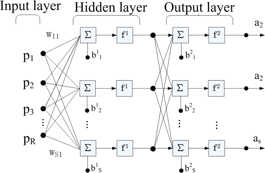
Back-propagation neural network.

Repeat phases 1 and 2 until the performance of the network is satisfactory. The complete algorithm for a three-layer network (only one hidden layer) is presented in Figure 4.

Figure 4.

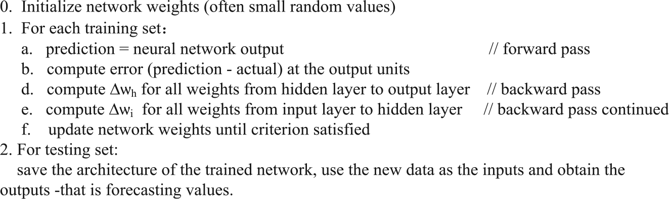
Back-propagation algorithm.

At present, there is no exact formulation to calculate the number of neurons in the input layer and the hidden layer. To optimize the prediction structures, a vast range of optimization tests must be conducted. In this article, BP neural network with 16 input neurons is the most appropriate to represent the traffic speed data of the consecutive Mondays by iterative trial. Of the 16 input neurons, 10 accepted the data before the current time, and others received historical data which were obtained at the same time on the previous day. The model is not retrained at the other location. This decision was made based on the fact that it would be highly unlikely that so many skilled personnel will be able to train neural network at different sites.

Nonparametric regression model

Nonparametric regression performs in a sense that it requires less computation and data overhead the ARIMA model and BP model. This approach does not need any prior training but instead performs prediction based on a group of similar past cases in the history database around the current input state at prediction time.

The similar past cases are referred as the nearest neighbors. In this research, a typical nonparametric regression method k nearest neighbors (KNN) is utilized, in which the underlying principle is to choose the KNN based on a distance measure, such as Euclidean distance.²¹ However, a suitable value for k must be determined by several attempts and then the one that gives the smallest prediction error is chosen.²² Once the neighbors are identified, the prediction is a weighted average of the KNN. The value of weight is then determined by the inverse of their distance. The complete algorithm is presented in Figure 5.

Figure 5.

Nonparametric regression algorithm.

In this research, the state vector $X (t)$ of the traffic speed data can be written as

X (t) = [x (t), x (t - 1), x (t - 2), x (t - 3)]

(2)

where x(t) is the traffic speed at the current time t, x(t − 1) is the traffic speed during the previous 5-min interval, and x(t + 1) is defined as the output of X(t). The data collected through the 10-month period constitute the development database.

Model comparisons

Performance indices

In order to fully evaluate the performance and potential for field implementation of the three forecasting approaches, a performance index system is established, as shown in Figure 6. The performance is evaluated in terms of two parts: quantitative index and qualitative index. The quantitative index consists of four components: absolute error (AE), root mean square error (RMSE), error distribution, and model portability. The qualitative index refers to the ease of implementing a forecasting model, which is evaluated based on the personal experience gained in developing the models.

Figure 6.

Performance indices.

AE

The AE describes how much the predicted values deviate from the actual values. To measure the statistical significance of difference between absolute average errors of the models, the Wilcoxon signed-rank test is used (Figure 7). The nonparametric statistical hypothesis test is used¹⁵ when comparing paired sample cases which are not normally distributed.²³ In this research, the pairs can be defined as the AE experienced by the two models at a given prediction time. In general, the test procedure of the Wilcoxon signed-rank test can be seen in Figure 7. Tables 1 –3 describe the results of the Wilcoxon signed-rank test in Jianguomen Bridge.

Figure 7.

Procedure of the Wilcoxon signed-rank test.

Table 1.

Wilcoxon signed-rank tests—morning peak.

Null hypothesis	Alternative hypothesis	Z-statistical	α = 0.05	Preferred model
$μ_{AR} - μ_{NNw} = 0$	$μ_{AR} - μ_{NNw} > 0$	−1.63	Reject H₀	ARIMA
$μ_{AR} - μ_{KNN} = 0$	$μ_{AR} - μ_{KNN} > 0$	6.98	Reject H₀	KNN
$μ_{NNw} - μ_{KNN} = 0$	$μ_{NNw} - μ_{KNN} > 0$	5.25	Reject H₀	KNN

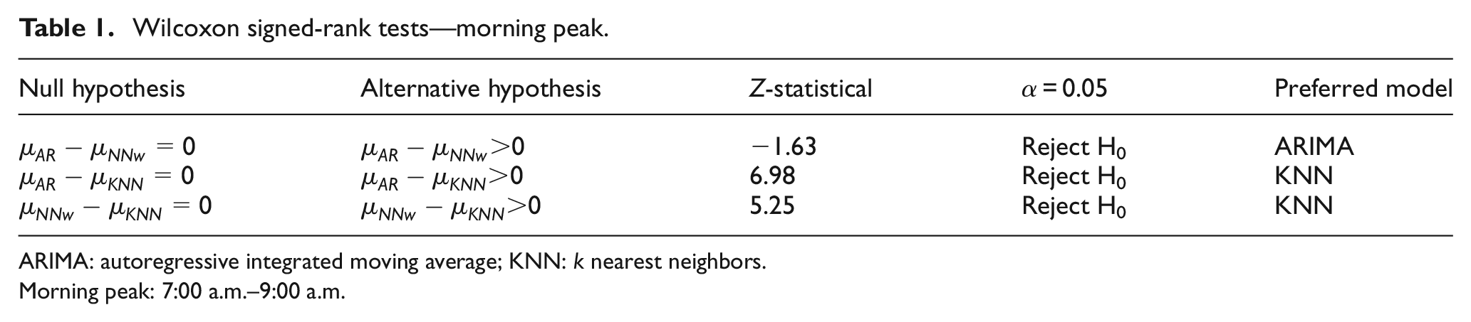
ARIMA: autoregressive integrated moving average; KNN: k nearest neighbors.

Morning peak: 7:00 a.m.–9:00 a.m.

Table 2.

Wilcoxon signed-rank tests—nonpeak.

Null hypothesis	Alternative hypothesis	Z-statistical	α = 0.05	Preferred model
$μ_{AR} - μ_{NNw} = 0$	$μ_{AR} - μ_{NNw} > 0$	−1.06	Accept H₀	Equal
$μ_{AR} - μ_{KNN} = 0$	$μ_{AR} - μ_{KNN} > 0$	−0.44	Accept H₀	Equal
$μ_{NNw} - μ_{KNN} = 0$	$μ_{NNw} - μ_{KNN} > 0$	−0.84	Accept H₀	Equal

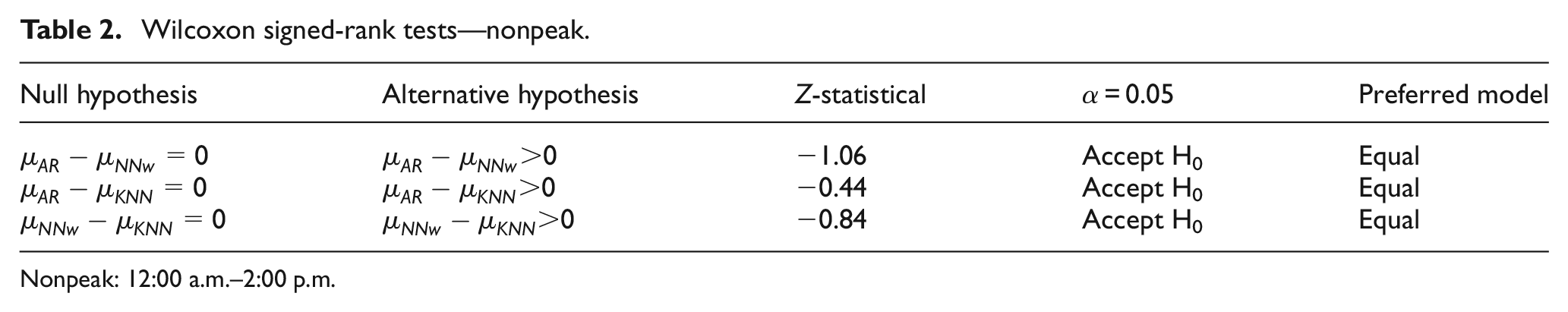
Nonpeak: 12:00 a.m.–2:00 p.m.

Table 3.

Wilcoxon signed-rank tests—evening peak.

Null hypothesis	Alternative hypothesis	Z-statistical	α = 0.05	Preferred model
$μ_{AR} - μ_{NNw} = 0$	$μ_{AR} - μ_{NNw} > 0$	−3.05	Reject H₀	ARIMA
$μ_{AR} - μ_{KNN} = 0$	$μ_{AR} - μ_{KNN} > 0$	1.52	Reject H₀	KNN
$μ_{NNw} - μ_{KNN} = 0$	$μ_{NNw} - μ_{KNN} > 0$	3.35	Reject H₀	KNN

ARIMA: autoregressive integrated moving average; KNN: k nearest neighbors.

Evening peak: 5:00 p.m.–7:00 p.m.

Tables 1 –3 illustrate the results for the Wilcoxon signed-rank test. It is clear that average AEs by the KNN model are significantly lower than those from the other two models in morning peak and evening peak. However, they are statistically equal in nonpeak time.

RMSE

The RMSE is defined as the square root of the mean of the squares of the deviations between the actual and predicted values, as illustrated below. RMSE is a good measure of accuracy. It only compares forecasting errors of different models for a particular variable but not between variables, as it is scale dependent.²⁴ The RMSE serves to magnify the relative difference between errors because of the square, so it is helpful to estimate which model carries the larger error point. The RMSE of Jianguomen Bridge on the three tests is represented in Figure 8

RMSE = \sqrt{\frac{1}{N} \sum_{i = 1}^{N} {[x (t) - \hat{x} (t)]}^{2}}

(3)

Figure 8.

RMSE comparison.

where $\hat{x} (t)$ is the predicted value of actual value $x (t)$ and N is the total number of predicted values.

As shown in Figure 8, the BP model gives the largest error in all three tests, whereas the ARIMA model and KNN model lead to comparable error results on morning peak and evening peak, and ARIMA model is more accurate on nonpeak time. In other words, the BP model has the larger error point. It is most likely due to the network training process.

Distribution of error

The distribution of error serves to evaluate the proportion of predicted values within a specified threshold (Table 4), and it can be used to describe how reliable the predicted values are. In this article, two thresholds are defined: predicted values higher and lower than 10% of the actual values. Moreover, the higher the proportion, the better the prediction accuracy.

Table 4.

Error distribution.

Model	Morning peak (%)	Nonpeak (%)	Evening peak (%)	Average (%)
ARIMA	36	48	24	36
BP	28	48	18	31
KNN	38	48	58	48

ARIMA: autoregressive integrated moving average; BP: back-propagation; KNN: k nearest neighbors.

Comparing the error distribution in Table 4, the BP model gives the least accurate results, whereas the error distributions of the ARIMA model and KNN model are almost equal on morning peak. However, three models have the same error results on nonpeak time. On the whole, the KNN model has the highest proportion at 48%, as compared to 36% and 31% for the other two models.

Model portability

Model portability refers to the consistent performance of a model at different sites. Once a model is developed for one site, it should perform comparably at other sites where it is deployed. This component of the quantitative performance index is measured by comparing the difference in the errors experienced by the three models at two different sites. The errors are represented in Tables 5 –7.

Table 5.

Error measures—morning peak.

Model	MAE	RMSE
ARIMA	30.09^a, 9.26^b	20.67^a, 15.21^b
BP	29.92^a, 9.92^b	18.73^a, 17.29^b
KNN	9.02^a, 8.94^b	13.25^a, 14.05^b

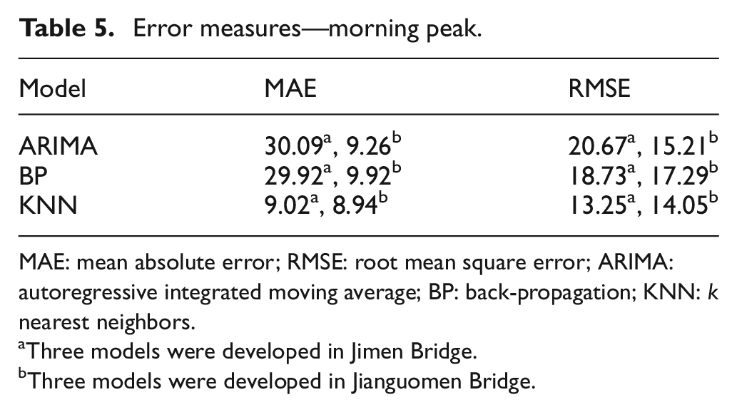
MAE: mean absolute error; RMSE: root mean square error; ARIMA: autoregressive integrated moving average; BP: back-propagation; KNN: k nearest neighbors.

Three models were developed in Jimen Bridge.

Three models were developed in Jianguomen Bridge.

Table 6.

Error measures—nonpeak.

Model	MAE	RMSE
ARIMA	35.67^a, 8.06^b	17.98^a, 9.93^b
BP	39.94^a, 9.94^b	18.56^a, 13.57^b
KNN	9.06^a, 7.53^b	13.57^a, 12.78^b

MAE: mean absolute error; RMSE: root mean square error; ARIMA: autoregressive integrated moving average; BP: back-propagation; KNN: k nearest neighbors.

Three models were developed in Jimen Bridge.

Three models were developed in Jianguomen Bridge.

Table 7.

Error measures—evening peak.

Model	MAE	RMSE
ARIMA	29.71^a, 6.71^b	20.08^a, 7.83^b
BP	40.69^a, 12.81^b	30.76^a, 19.57^b
KNN	5.79^a, 4.46^b	7.53^a, 7.28^b

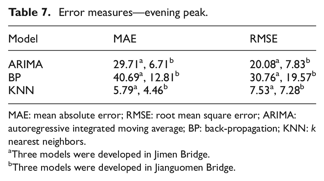
MAE: mean absolute error; RMSE: root mean square error; ARIMA: autoregressive integrated moving average; BP: back-propagation; KNN: k nearest neighbors.

Three models were developed in Jimen Bridge.

Three models were developed in Jianguomen Bridge.

As shown in Tables 5 –7, the ARIMA model and the BP model experience significantly high error at Jimen Bridge. The average MAE value and RMSE value of ARIMA model on three tests is 3.97 times and 1.78 times higher than those for Jianguomen Bridge, respectively. Similarly, the BP model gives 3.38 times and 1.35 times higher error than those for Jianguomen Bridge in MAE and RMSE values. However, the errors of KNN model are comparable to that calculated at Jianguomen Bridge on three tests.

The results suggest that the ARIMA model and the BP model exhibit a poor portability, as a result of the fact that different sites have different traffic characteristics over the same data collection period. Fitting parameters and training networks need to be conducted at a new site. However, because of the capability to exploit information contained with a large set of data, in which similar states always exist, KNN model thus has the best portability.

Ease of model implementation

The ease of implementing a traffic flow forecasting model carries a significant impact in ITS. Simple operation does not require a large number of professionals to conduct models for different sites. Otherwise, if the modeling need complicated parameter definition and training process, it is likely that the model will never be generalized. This qualitative performance index has certain subjectivity (Table 8).

Table 8.

Implementation comparison.

Model	ARIMA	BP	KNN
Implementation	Complex	More complex	Simple

ARIMA: autoregressive integrated moving average; BP: back-propagation; KNN: k nearest neighbors.

Comparative analysis

In order to describe the extent of fluctuation in the data, the CV was used, which is defined as the ratio of the standard deviation (SD) to the mean.²⁵ This parameter was used in place of a more traditional statistics parameter of SD because the SD of data must always be understood in the context of the mean of the data. In contrast, the actual value of the CV is independent of the unit in which the measurement has been taken, so it is a dimensionless number. For comparison between datasets with widely different means, the CV was selected to describe fluctuation of the data. The CV of actual values is shown in Table 9. Moreover, the smaller the CV, the smaller the fluctuation of data.

Table 9.

CV comparison.

CV	Morning peak	Nonpeak	Evening peak
Jianguomen Bridge	1.06	0.33	0.82
Jimen Bridge	1.03	0.42	0.81

CV: coefficient of variation.

On examining Tables 1 –3, the results illustrate that KNN model outperforms the other models when the time series fluctuate considerably (morning peak and evening peak), and the performance of the three models is similar when the time series fluctuate gently (nonpeak). Similarly, Table 4 describes the distribution of error at the Jianguomen Bridge site, and the three models produce identical accuracy on nonpeak because of the lower CV.

As shown in Tables 5 –7, the results clearly show that the ARIMA model and BP model are not portable. They were developed at a different site (Jimen Bridge), where the performance deteriorates in the estimation of future traffic data because of a lack of capability to capture a “universal” underlying relationship between the system’s current status and its future status. However, it is clear that for the models to be effective, they must be developed with data collected at each site where they will be used.

It is clear that the ARIMA model and BP model require extensive data calibration, but the KNN model can be employed without such overhead, and it can be implemented easily. However, the weakness of the KNN model is the complexity of the search to identify the “neighbors.” On the whole, the KNN model has the most accurate prediction results, compared to the ARIMA model and BP model.

Conclusion

This article discussed three representative short-time prediction models of the traffic speed data at 5-min interval. They are ARIMA, neutral network, and nonparametric regression. To evaluate the performance and potential for field implementation of these models, a performance index system including AE, RMSE, error distribution, and model portability is introduced. The performance of the three models is compared with real-life data in Beijing.

The results suggest that the ARIMA model, BP model, and KNN model will have the same prediction accuracy when the time series fluctuate gently. However, the KNN model seems to be more robust for extensive applications in practice.

The three models produce very similar level of error on nonpeak time. However, the KNN model experienced significantly less error than the other two models when the time series fluctuate dramatically. Moreover, the KNN model does not require parameter fitting and structure training, which makes it easier to implement.

Furthermore, the KNN model was successfully applied at multiple sites. This is demonstrated by the comparable error characteristics of the model produced in the development tests at two different sites. This advantage is most likely due to the theoretical foundation that the model can exploit information contained with a large set of data. Finally, if the time series vary gently and have a large number of professionals, the three models are all comparable. Otherwise, the KNN model is a better choice.

The results presented in this article point to the potential for further research. Because the KNN model requires more complex process to identify the “neighbors,” it is necessary to investigate suitable means to improve the search speed. Besides traffic conditions are associated with various factors, more data in terms of traffic volume and occupancy should be included to develop a multivariate nonparametric regression.

Footnotes

Academic Editor: Xiaobei Jiang

Declaration of conflicting interests

The author(s) declared no potential conflicts of interest with respect to the research, authorship, and/or publication of this article.

Funding

The author(s) disclosed receipt of the following financial support for the research, authorship, and/or publication of this article: This research is supported by National Basic Research Program of China (2012CB725406) and National Natural Science Foundation of China (71131001).

References

Wang

Shang

Zhao

. A new traffic speed forecasting method based on bi-pattern recognition. Fluct Noise Lett 2011; 10: 59–75.

Joueiai

Van

Hoogendoorn

. Multi-scale traffic flow modeling in mixed networks. Transp Res Record 2014; 2421: 142–150.

Liu

. Application of chaos and neural network in power load forecasting. Discrete Dyn Nat Soc 2011; 2011: 597634.

. Research and application of the Beijing road traffic prediction system. Discrete Dyn Nat Soc 2014; 2014: 316032.

Cheng

Haworth

Wang

. Spatio-temporal autocorrelation of road network data. J Geogr Syst 2012; 14: 389–413.

Sun

Wang

Zhao

. Predicting cooling loads for the next 24 hours based on general regression neural network: methods and results. Adv Mech Eng 2013; 2013: 954185.

Haworth

Cheng

. Non-parametric regression for space–time forecasting under missing data. Comput Environ Urban 2012; 36: 538–550.

Meng

Shao

Wong

. A two-stage short-term traffic flow prediction method based on AVL and AKNN techniques. J Cent South Univ 2015; 22: 779–786.

Karlaftis

Vlahogianni

. Statistical methods versus neural networks in transportation research: differences, similarities and some insights. Transport Res C: Emer 2011; 19: 387–399.

10.

Kirby

Watson

Dougherty

. Should we use neural networks or statistical models for short-term motorway traffic forecasting? Int J Forecasting 1997; 13: 43–50.

11.

Abdi

Moshiri

Abdulhai

. Forecasting of short-term traffic-flow based on improved neurofuzzy models via emotional temporal difference learning algorithm. Eng Appl Artif Intel 2012; 25: 1022–1042.

12.

Smith

Williams

Oswald

. Comparison of parametric and nonparametric models for traffic flow forecasting. Transport Res C: Emer 2002; 10: 303–321.

13.

Tang

William

Pan

. Comparison of four modeling techniques for short-term AADT forecasting in Hong Kong. J Transp Eng 2003; 129: 271–277.

14.

William

Tang

Tam

. Comparison of two non-parametric models for daily traffic forecasting in Hong Kong. J Forecasting 2006; 25: 173–192.

15.

Smith

Demetsky

. Traffic flow forecasting: comparison of modeling approaches. J Transp Eng 1997; 123: 261–266.

16.

Vlahogianni

Golias

Karlaftis

. Short-term traffic forecasting: overview of objectives and methods. Transport Rev 2004; 24: 533–557.

17.

Vlahogianni

Karlaftis

Golias

. Short-term traffic forecasting: where we are and where we’re going. Transport Res C: Emer 2014; 43: 3–19.

18.

Wang

Liu

. Mean velocity prediction information feedback strategy in two-route systems under ATIS. Adv Mech Eng 2015; 7: 640416.

19.

Lee

Fambro

. Application of subset autoregressive integrated moving average model for short-term freeway traffic volume forecasting. Transp Res Record 1999; 1678: 179–188.

20.

Box

Jenkins

Reinsel

. Time series analysis: forecasting and control. New York, NY: John Wiley & Sons, 2011.

21.

Hardle

. Applied nonparametric regression. Cambridge: Cambridge University Press, 1990.

22.

Sun

Liu

Zhu

. Traffic flow forecasting based on large scale traffic flow data. J Transp Syst Eng Inf Technol 2013; 13: 121–125.

23.

Lowry

. Concepts and applications of inferential statistics, 1998, http://www.e-booksdirectory.com/details.php?ebook=80

24.

Hyndman

Koehler

. Another look at measures of forecast accuracy. Int J Forecasting 2006; 22: 679–688.

25.

Stevens

. On the theory of scales of measurement. Science 1946; 103: 677–680.

Comparative analysis for traffic flow forecasting models with real-life data in Beijing

Abstract

Keywords

Introduction

Data collection

Study location

Data description

Models

ARIMA model

Back-propagation neural network model

Nonparametric regression model

Model comparisons

Performance indices

AE

RMSE

Distribution of error

Model portability

Ease of model implementation

Comparative analysis

Conclusion

Footnotes

Declaration of conflicting interests

Funding

References