Sage Journals: Discover world-class research

Abstract

The applications of pressure work, pressure-dilatation, and dilatation-dissipation (Sarkar, Zeman, and Wilcox) models to hypersonic boundary flows are investigated. The flat plate boundary layer flows of Mach number 5–11 and shock wave/boundary layer interactions of compression corners are simulated numerically. For the flat plate boundary layer flows, original turbulence models overestimate the heat flux with Mach number high up to 10, and compressibility corrections applied to turbulence models lead to a decrease in friction coefficients and heating rates. The pressure work and pressure-dilatation models yield the better results. Among the three dilatation-dissipation models, Sarkar and Wilcox corrections present larger deviations from the experiment measurement, while Zeman correction can achieve acceptable results. For hypersonic compression corner flows, due to the evident increase of turbulence Mach number in separation zone, compressibility corrections make the separation areas larger, thus cannot improve the accuracy of calculated results. It is unreasonable that compressibility corrections take effect in separation zone. Density-corrected model by Catris and Aupoix is suitable for shock wave/boundary layer interaction flows which can improve the simulation accuracy of the peak heating and have a little influence on separation zone.

Keywords

Turbulence models compressibility corrections hypersonic flat plate boundary layer compression corners shock wave/boundary layer interaction

Introduction

With the rapid development of hypersonic vehicles, accurate prediction of the skin friction and heat flux is critical for the vehicle design. Numerical simulation is a major method for hypersonic boundary flows and turbulence model is one of the most important factors affecting computational accuracy. The most common turbulence models are set up for incompressible flows. When they are applied to hypersonic compressible flows, compressibility corrections are need. Compressibility corrections are performed by two ways. The one is the modification of mean flow equations with consideration for the variations of mean density using Favre averaging. The other is adding the compressibility corrections in turbulence kinetic energy (TKE) equation by modeling the extra compressible terms appeared explicitly with the consideration for compressible effects on turbulence structure itself.

For the simulations of wall-bounded turbulence flows, explicit compressibility corrections are not considered to be important up to a Mach number of at least 5. Morkovin hypothesis¹ states that the fluctuations of thermodynamic variables such as pressure, density, and temperature are relatively small compared with the mean variables for Mach number up to about 5. The compressibility is mainly expressed as the effect on mean flow. The compressible turbulence models can be obtained by direct varied-density extension of incompressible turbulence models. However, with the gradual increase of Mach number, compressibility effects on turbulence structure become significant and explicit compressible terms in turbulence kinetic equation cannot be ignored.

In the Favre averaging framework, three compressible terms arise in TKE equation compared with its incompressible form. They are dilatation-dissipation, pressure-dilatation, and pressure work.>2 The compressibility corrections are mainly for these three terms. There are plenty of investigations on compressibility corrections and some methods^3–7 are presented. At the early stage, the compressibility investigations are focused on the mixing layer and the decrease in growth rate in the mixing layer with increasing Mach number is observed in experiments and direct numerical simulation (DNS). Compressibility corrections are devised to deal with the effects of compressibility on the dissipation rate of the TKE. Sarkar et al.,³ Wilcox,⁴ and Zeman⁵ present compressibility correction separately for dilatation-dissipation term which are based on the turbulence Mach number. Sarkar et al.³ modeled the ratio of the dilatation-dissipation to the solenoidal dissipation as a function of the turbulence Mach number. Zeman⁵ takes the compressibility effect into account with the consideration for dissipation by shocklet structure in compressible flows and compares the variation of mixing layer growth rate as convective Mach number with experiments. Pressure-dilatation model proposed by Sarkar⁶ adds the pressure-dilatation term in k equation on the basis of turbulence Mach number similarly. Pressure work⁷ is the scalar product of Favre averaged velocity fluctuation and mean pressure gradient which is modeled by Speziale with gradient law. However, these compressibility corrections are mainly applied to free-shear or jet flows and the investigation of their applicability to compressible boundary layer flow is worthwhile.

Except the corrections for compressible terms in k equation, rapid compression fix is proposed by Coakley and Huang⁸ to improve predictions of flow separation in shock wave/boundary layer interaction. Turbulent length scale correction⁹ is devised to reduce the large overshoot in heat transfer rates near reattachment by introducing an upper bound on the turbulent length scale. Stress limiter¹⁰ suppresses the magnitude of the Reynolds shear stress when production of TKE exceeds its dissipation. But the stress limiter coefficients are chosen experientially.

In addition, Sarkar¹¹ finds that the decrease in TKE is due to the decrease in production term of TKE rather than dilatation compressibility effects in DNS results for shear layer flows. Sinha and Balasridhar¹² point out that the TKE will increase rapidly to an extremely high value across a shock wave resulting in an amplification of turbulent eddy viscosity. The various disputes indicate that compressible turbulence especially for hypersonic flows needs to be studied deeply.

In application aspect, Grasso and Falconi¹³ performed numerical simulations for two cases of flat plat and compression corner flows adopting the dilatation-dissipation, pressure-dilatation, pressure work corrections, and turbulence length scale correction synthetically in k-ε equations. The researches show that the compressibility corrections can contribute to reducing the peak heating. But the investigations do not evaluate the difference of various compressibility corrections in detail and numerical cases are relatively few. Rumsey¹⁴ studied the application of Wilcox and Zeman dilatation-dissipation correction to the flat plate boundary layer flows. But the computational results are lack of validation with experimental data and only compared with Van Driest correlations. The researches of separation flows are not carried out. Tu et al.¹⁵ analyze the accuracy for compression corners adopted pressure-dilatation by Sarkar and dilatation-dissipation by Wilcox with high-order numerical schemes. Liu¹⁶ gives a new approximation of pressure work and considers it to be important. Dong and Zhou¹⁷ evaluate the Baldwin-Lomax (BL) algebraic turbulence models for hypersonic flows and results show that the Prandtl number is not constant in DNS. The turbulent eddy viscosity computed by Spalart-Allmaras (SA) and k-ε models is overestimated while BL model underpredicts it in DNS results of flat plate by Li et al.¹⁸ at Mach 6.0. Catris and Aupoix¹⁹ propose a correction of the diffusion terms in turbulent models to make the models compatible with the logarithmic law for a compressible boundary layer.

At present, the influence of different compressibility corrections on simulation accuracy for hypersonic flows is not understood deeply. The systematic recognition does not form on how to use these models in numerical simulations. In this article, the application study is carried out for hypersonic boundary layer flows with the various compressibility correction models including dilatation-dissipation (Sarkar, Zeman, and Wilcox), pressure-dilatation, pressure work, rapid compression fix, and density-corrected model by Catris. First, compared with the experimental data of hypersonic flat plate turbulent boundary layer, the suitability of different compressibility correction models are assessed detailedly over a wide range of Mach numbers, and the effects on velocity profiles, friction, and heat transfer are evaluated. Secondly, compared with hypersonic compression corner experiments, the effects of compressibility corrections on separation zone size and heat transfer distribution are studied for shock wave/boundary layer interaction, and the physical mechanism of influence tendency is analyzed. Finally, the density-corrected model by Catris is studied.

Numerical methods

The numerical computations adopt ACANS (Aerodynamic, Combustion and Aerothermodynamic Numerical Simulation) finite difference program of National Laboratory of Computational Fluid Dynamics. The accuracy of ACANS finite difference code has been verified by several studies.^20,21 The governing equations are Favre averaged Navier–Stokes equations. The compressible turbulence models are fully coupled with the mean flow equations. The convection terms are computed by Advection Upstream Splitting Method by Pressure-based Weight functions (AUSMPW)²² scheme in conjunction with the Monotone Upstream-centered Scheme for Conservation Laws (MUSCL)²³ interpolation to achieve second-order accuracy. The viscous terms are discretized by second-order central difference scheme. Implicit Lower-Upper Symmetric Gauss-Seidel (LU-SGS)²⁴ method is used for time advancing. The k-ω shear stress transport (SST), k-ω models, and their compressible forms are applied to numerical computations.

Governing equations

The Favre averaged Navier–Stokes² equations for conservation of mass, momentum, and energy are as follows

\begin{array}{l} \frac{\partial ρ}{\partial t} + \frac{\partial}{\partial x_{j}} (ρ u_{j}) = 0 \\ \frac{\partial}{\partial t} (ρ u_{i}) + \frac{\partial}{\partial x_{j}} (ρ u_{j} u_{i}) = - \frac{\partial p}{\partial x_{i}} + \frac{\partial {\hat{τ}}_{j i}}{\partial x_{j}} \\ \frac{\partial}{\partial t} (ρ E) + \frac{\partial}{\partial x_{j}} ((ρ E + p) u_{j}) = \frac{\partial}{\partial x_{j}} \\ [u_{i} {\hat{τ}}_{j i} + (μ_{l} + σ_{k} μ_{t}) \frac{\partial k}{\partial x_{j}} + (\frac{μ_{l}}{\underset{l}{\Pr}} + \frac{μ_{t}}{\underset{t}{\Pr}}) \frac{\partial h}{\partial x_{j}}] \end{array}

(1)

where ρ, u_i, and p represent the density, cartesian velocity components, and pressure respectively; E is the total energy per unit mass; h is the enthalpy per unit mass; k is the TKE; Pr_l and Pr_t are molecular and turbulent Prandtl numbers; the shear stress terms ${\hat{τ}}_{ij}$ are composed of a laminar and a turbulent component as

{\hat{τ}}_{ij} = τ_{ij}^{L} + τ_{ij}^{T}

(2)

The laminar component is

τ_{ij}^{L} = 2 μ_{l} (S_{ij} - \frac{1}{3} \frac{\partial u_{k}}{\partial x_{k}} δ_{ij})

(3)

where µ_l is molecular viscosity and S_ij is the symmetric part of the mean strain tensor defined by

S_{ij} = 0.5 (\partial u_{i} / \partial x_{j} + \partial u_{j} / \partial x_{i})

(4)

The turbulent component is

τ_{ij}^{T} = 2 μ_{t} (S_{ij} - \frac{1}{3} \frac{\partial u_{k}}{\partial x_{k}} δ_{ij}) - 2 / 3 ρ k δ_{ij}

(5)

where µ_t is turbulent viscosity.

Compressible form of two-equation turbulence models

Compressibility corrections for k-ω SST turbulence model²⁵ are expressed as

\begin{array}{l} \frac{\partial (ρ k)}{\partial t} + \frac{\partial (ρ u_{j} k)}{\partial x_{j}} = P_{k} - β^{*} ρ ω k + \frac{\partial}{\partial x_{j}} [(μ + σ_{k} μ_{t}) \frac{\partial k}{\partial x_{j}}] + Π_{c 1} + Π_{c 2} \\ \frac{\partial (ρ ω)}{\partial t} + \frac{\partial (ρ u_{j} ω)}{\partial x_{j}} = \frac{α ρ}{μ_{t}} P_{k} - β ρ ω^{2} + \frac{\partial}{\partial x_{j}} [(μ + σ_{ω} μ_{t}) \frac{\partial ω}{\partial x_{j}}] \\ + 2 ρ (1 - F_{1}) \frac{σ_{ω 2}}{ω} \frac{\partial k}{\partial x_{j}} \frac{\partial ω}{\partial x_{j}} + Ψ_{c 1} + Ψ_{c 2} \end{array}

(6)

where ω is the specific dissipation rate; turbulence production term is defined as P_k = τ_ij∂u_i/∂x_j; F₁ is blending function; Π_c1 and Π_c2 are pressure work and pressure-dilatation terms respectively; Ψ_c1 and Ψ_c2 are the compressible terms derived from the Π_c1 and Π_c2 according to the correlation ε = β*ωk. The other terms and coefficients can be found in Menter.²⁵ The k-ω turbulence model² (1988a) has similar form and is not listed here.

Pressure work and pressure-dilatation corrections

In TKE equation, pressure work and pressure-dilatation are described as

Π_{c 1} = \bar{{u ″}_{i}} \frac{\partial p}{\partial x_{i}} Π_{c 2} = \bar{p' \frac{\partial {u ″}_{i}}{\partial x_{i}}}

(7)

The pressure work⁷ is modeled as

Π_{c 1} = - \frac{μ_{t}}{ρ^{2}} \frac{1}{σ_{ρ}} \frac{\partial ρ}{\partial x_{j}} \frac{\partial p}{\partial x_{j}}

(8)

where σ_ρ = 0.5.

Pressure-dilatation⁶ is modeled as

Π_{c 2} = (- α_{2} P_{k} + α_{3} ρ ε) M_{T}^{2}

(9)

where α₂ = 0.4, α₃ = 0.2, and M_T is the turbulence Mach number defined by

M_{T} = \sqrt{\frac{2 k}{a^{2}}}

(10)

where a is the speed of sound and k is TKE.

When the above corrections of pressure work and pressure-dilatation are applied to k-ω SST and k-ω turbulence models, the new compressibility terms ψ_c1 and ψ_c2 appear in the ω equation according to the correlation ε = β^*ωk

Ψ_{c 1} = - \frac{Π_{c 1}}{ν_{t}} Ψ_{c 2} = - \frac{Π_{c 2}}{ν_{t}}

(11)

where ν_t = µ_t/ρ is the turbulent kinematic viscosity.

Dilatation-dissipation correction

The dissipation terms are modeled as incompressible dissipation ε_s and dilatation-dissipation ε_d where ε_s employs the original form. Sarkar et al.,³ Wilcox,⁴ and Zeman⁵ proposed compressibility corrections for dilatation-dissipation term based on the turbulence Mach number. The original coefficients of dissipation term are modified as

\begin{matrix} β_{c}^{*} = β^{*} [1 + ξ^{*} F (M_{T})] \\ β_{c} = β - β^{*} ξ^{*} F (M_{T}) \end{matrix}

(12)

1. Sarkar et al.³ model

ξ^{*} = 1 F (M_{T}) = M_{T}^{2}

(13)

2. Zeman⁵ model

\begin{matrix} ξ^{*} = \frac{3}{4} \\ F (M_{T}) = [1 - e^{- \frac{1}{2} (γ + 1) {(M_{t} - M_{t_{0}})}^{2} / Λ^{2}}] H (M_{t} - M_{t_{0}}) \\ M_{t_{0}} = 0.25 \sqrt{\frac{2}{(γ + 1)}} \end{matrix}

(14)

where γ is the specific-heat ratio and H(x) is Heaviside step function with $Λ = 0.66$ .

3. Wilcox⁴ model

ξ^{*} = 2 F (M_{T}) = (M_{T}^{2} - M_{T_{0}}^{2}) H (M_{T} - M_{T_{0}})

(15)

where $M_{T_{0}}$ is equal to 0.25.

Profiles of ξ*F(M_T) are shown as a function of M_T for three dilatation-dissipation corrections in Figure 1. It is shown that Sarkar correction is enabled active for all the M_T. But the Zeman and Wilcox corrections only work when the M_T is greater than a threshold value $M_{T_{0}}$ of 0.22 and 0.25, respectively. The correction level of Zeman correction is lower than that of Wilcox and Sarkar models. The correction level of Sarkar model is the greatest when M_T is less than a value of about 0.4 while Wilcox model has the largest correction level with M_T greater than 0.4.

Figure 1.

Variation of ξ*F(M_T) for three dilatation-dissipation corrections.

Synthetical correction

Grasso and Falconi¹³ adopt the dilatation-dissipation, pressure-dilatation, pressure work correction, turbulence length scale correction, and Karman constant modification synthetically in k-ε equations. The dilatation-dissipation formula in Grasso and Falconi¹³ is as follows

\begin{matrix} ξ^{*} = 0.4 \\ F (M_{T}) = [1 - e^{- {(M_{T} - M_{T_{0}})}^{2} / {0.8}^{2}}] H (M_{T} - M_{T_{0}}) \\ M_{T_{0}} = 0.3 \end{matrix}

(16)

Turbulence length scale correction

The peak heating is generally overpredicted because ω is very small leading to rapid increasing of turbulence length scale near reattachment. This does not exist in zero or one equations in which turbulence length scale is defined with algebraic correlation. Vuong and Coakley⁹ modify this as

l = min (κ \sqrt{a_{1}} d; \sqrt{k} / ω)

(17)

where a₁ = 0.31, κ = 0.41, and d is the normal distance from the wall. The turbulence viscosity is computed by the following equation according the formulation $ω = \sqrt{k} / l$

μ_{t} = min (μ_{t, org}, ρ κ d \sqrt{a_{1} k})

(18)

Rapid compression fix

The rapid compression fix⁸ puts forward for separation zone size and wall pressure prediction by ensuring that the turbulent length scale does not change too quickly when undergoing rapid compression. In this method, the production term in the ω equation

\begin{matrix} \frac{γ ρ}{μ_{t}} P_{k} = \frac{γ ρ}{μ_{t}} τ_{ij} \frac{\partial u_{i}}{\partial x_{j}} = \frac{γ ρ}{μ_{t}} [μ_{t} {\bar{S}}^{2} - \frac{2}{3} ρ k δ_{ij} \frac{\partial u_{i}}{\partial x_{j}}] \\ = γ ρ {\bar{S}}^{2} - \frac{2}{3} γ ρ ω \frac{\partial u_{k}}{\partial x_{k}} \end{matrix}

(19)

is modified as

\frac{γ ρ}{μ_{t}} P_{k} = γ ρ {\bar{S}}^{2} - \frac{4}{3} ρ ω \frac{\partial u_{k}}{\partial x_{k}}

(20)

where γ is the specific-heat ratio and ${\bar{S}}^{2}$ is defined by

{\bar{S}}^{2} = (\frac{\partial u_{i}}{\partial x_{j}} + \frac{\partial u_{j}}{\partial x_{i}} - \frac{2}{3} \frac{\partial u_{k}}{\partial x_{k}} δ_{i j}) \frac{\partial u_{i}}{\partial x_{j}} = (\frac{\partial u_{i}}{\partial x_{j}} + \frac{\partial u_{j}}{\partial x_{i}}) \frac{\partial u_{i}}{\partial x_{j}} - \frac{2}{3} {(\frac{\partial u_{k}}{\partial x_{k}})}^{2}

Catris and Aupoix correction

Catris and Aupoix¹⁹ proposed a modification of the diffusion terms to account for density gradients and retrieve the logarithmic law for hypersonic boundary layers. In this article, the correction for k-ω model is as follows

\begin{array}{l} \frac{\partial (ρ k)}{\partial t} + \frac{\partial (ρ u_{j} k)}{\partial x_{j}} = P_{k} - β^{*} ρ ω k + \frac{\partial}{\partial x_{j}} [(\frac{μ + σ_{k} μ_{t}}{ρ}) \frac{\partial (ρ k)}{\partial x_{j}}] \\ \frac{\partial (ρ ω)}{\partial t} + \frac{\partial (ρ u_{j} ω)}{\partial x_{j}} = \frac{α ρ}{μ_{t}} P_{k} - β ρ ω^{2} + \frac{\partial}{\partial x_{j}} [(\frac{μ + σ_{ω} μ_{t}}{\sqrt{ρ}}) \frac{\partial (\sqrt{ρ} ω)}{\partial x_{j}}] \end{array}

(21)

Results and discussions

The numerical simulations are executed for attached flat plate flow and shock wave/boundary layer interaction with the above compressibility corrections. For convenience, the results of all kinds of compressibility corrections in the following figures have simplified notations. For example, pressure work is denoted by “Press-work”; pressure-dilatation denoted by “Press-dilatation”; dilatation-dissipation proposed by Sarkar, Wilcox, and Zeman denoted by “D-D_S,”“D-D_W,” and “D-D_Z”; the method proposed by Grasso and Falconi¹³ denoted by “all”; Grasso and Falconi¹³ method with turbulence length scale and Karman constant modification denoted by “all + length scale + Karman”; and the method proposed by Catris and Aupoix denoted by “density-corrected model.”

Compressibility corrections

Hypersonic flat plate boundary layer

The numerical cases of turbulence boundary layer on a flat plate are selected for evaluating the suitability of compressibility corrections for hypersonic attached flows. The measured friction coefficients and Stanton number are given in the experiments.^26,27 The Mach number is in the range of 5–11. Stanton number is defined as St = q_w/ρ_∞ U_∞ C_p(T_aw − T_w), where ρ_∞ and U_∞ are freestream density and velocity, respectively; C_p is the specific heat at constant pressure; T_w is the wall temperature; and T_aw is the recovery temperature defined by T_aw = T_∞*(1 + r(γ − 1)/2*Ma²) where r is recovery factor and γ is the specific heat ratio. In the experiment, the boundary layer transition occurs near the position of x = 0.1 m for Mach number 5.0 case and x = 0.2 m for the other cases. To simulate the transition in computation, the laminar simulation (µ_t is forced to be zero over all the domain prior to transition by hard-coded into the program) is adopted, while afterward the turbulent simulation works.

Numerical simulation is performed for seven cases of flat plate boundary layers with Mach numbers ranging from 5 to 11 and T_w/T_aw between 0.19 and 0.80. The detailed flow conditions are given in Table 1. No-slip and isothermal wall boundary conditions are used. The inflow and top boundary is initiated with incoming airstream. The outflow boundary condition is treated using extrapolation from the interior of the domain.

Table 1.

Computation conditions for the flat plate cases.

Item	Ma	T _∞ (K)	T_w (K)	T_w/T_aw	Re (m)
1	5.0	68.79	300	0.80	37 × 10⁶
2	7.712	80.8	296.1	0.32	16.4 × 10⁷
3	7.97	71.7	291.5	0.33	56.5 × 10⁶
4	7.982	108.6	292.2	0.22	58.5 × 10⁶
5	8.324	71.4	294.3	0.31	20.44 × 10⁷
6	10.6	67	296.1	0.21	36.94 × 10⁶
7	11.1	64	296.7	0.19	57.5 × 10⁶

A grid study for the M_∞ = 5 flat plate case was conducted using the SST model on two sets of grids of 257 × 129 (Figure 2) and 513 × 257. The y⁺ of two sets of grid is set to be less than 1. The wall pressure and the heat flux acquired from the two sets of grids are shown in Figure 3. It can be seen that there is no evident difference between the two results. Then the 257 × 129 grid as shown in Figure 2 is chosen for further study.

Figure 2.

Computation grid for the flat plate case.

Figure 3.

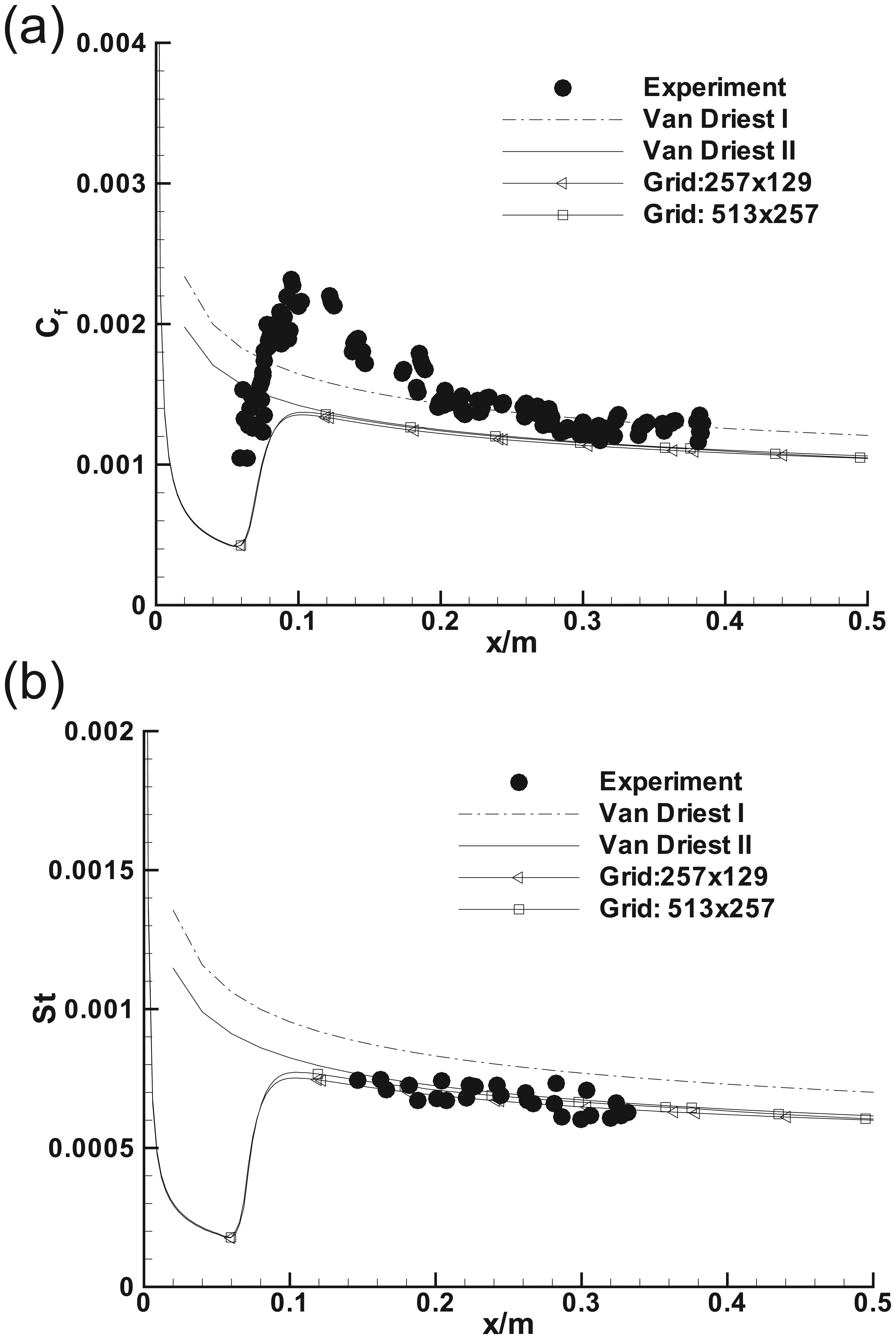
Grid study of friction coefficient and Stanton number for M_∞ = 5 using SST on two sets of grids: (a) friction coefficient and (b) Stanton number.

Profiles of turbulence Mach number are shown as a function of y in the boundary layer at the exit for several different cases in Figure 4. It is shown that the maximum level was only about 0.28 when Mach number is 5; the peak M_T arrives at 0.34 when Mach number goes up to about 8; and the peak M_T reaches approximately 0.46 with the increasing Mach number up to about 10. However, the M_T increases gradually as wall temperature decreases from T_w/T_aw = 0.31 to 0.21 with almost the same Mach numbers. For example, the M_T in test case 3 is smaller than that in test case 4. Additionally, it can be seen that M_T increases gradually with the decrease of Reynolds number at the same wall temperature but decreasing Mach numbers. For example, M_T in test case 3 is greater than that in test case 5.

Figure 4.

M_T profile at the exit.

Typical flat plate test cases for M_∞ = 5, 8.324, and 11.1 extracted from Table 1 are performed separately. Figures 5 –7 present the calculated friction and heat transfer. Van Driest correlation and the experiments are also given for validation. It is shown that the friction coefficients predicted by Van Driest II²⁸ is closer to the experiment data in comparison with the Van Driest I²⁹ solution. The theoretical St is obtained by Reynolds analogy correlation and Reynolds analogy factor is 1.16. Figures 5 and 6 indicate that original SST model is suitable for the flat plate boundary layer flow for Mach number ranging from 5 to 8. The calculated friction and heat transfer are in agreement with the experimental data. However, as the Mach number is greater than 10, an evident deviation of calculated results from experiment data takes place as shown in Figure 7. The friction coefficient predicted by SST model takes on little difference compared with that of the experiments while the heat transfer is overpredicted. The Van Driest transform serves as a verification check by comparing the transformed, incompressible velocity profile to the classical incompressible result with u⁺ = y⁺ in the near wall region and u⁺ = ln(y⁺)/0.41 + 5.5 for log-layer. The transformed velocity profiles for different Mach numbers are presented in Figures 5 –7(c). All the results follow the inner law variation in viscous sublayer and are in acceptable agreement with the classical limit in the log-law region at Mach about 5 and 8. At Mach 11.1, there is a derivation between incompressible velocity profile and calculated results in the log-law region. Therefore, compressibility corrections are needed.

Figure 5.

Results of flat plate case 1 by SST turbulence model and its compressibility versions: (a) friction coefficient, (b) Stanton number, and (c) u⁺ profile at exit location.

Figure 6.

Results of flat plate case 5 by SST turbulence model and its compressibility versions: (a) friction coefficient, (b) Stanton number, and (c) u⁺ profile at exit location.

Figure 7.

Results of flat plate case 7 by SST turbulence model and its compressibility versions: (a) friction coefficient (b) Stanton number, and (c) u⁺ profile at exit location.

First of all, the influence of compressibility corrections on calculated results is analyzed. The transformed velocity profiles by compressibility corrections show larger disagreement with the incompressible distributions in log-law region. It can be seen that the velocity profile of “D-D_S” is far above the incompressible velocity profile in log-law region. “Press-dilatation” and “D-D_Z” predict almost the same deviation from the incompressible logarithmic law while the “D-D_S” has the larger one. The changes of velocity profiles are the smallest for “Pressure-work” among all the compressibility corrections.

The dilatation-dissipation and “Press-dilatation” models are both constructed on the M_T. In turbulence boundary layers where the M_T value is large, they take effect. For equilibrium boundary layers, ${| α_{2} P |}_{k} > α_{3} ρ ε$ in equation (9), so the “Press-dilatation” reduces the production term of TKE. Consequently, the turbulent viscosity decreases. The “Press-work” contributes to reduce the TKE in the large pressure gradient region. The values of the two terms “Press-dilatation” and “Press-work” can be positive or negative. Therefore, from the aspect of the influence region, the “Press-work” has the greatest possibility to exhibit the least effect on calculated results by qualitative analysis.

All the corrections make friction coefficient and heat transfer decrease and the effects become more evident with the increasing Mach numbers. The reason is that these corrections reduce the turbulent viscosity. The effect of pressure work is the least, then the “Press-dilatation” and “D-D_Z” have the slightly larger effect, and the correction level of “D-D_S” dilatation-dissipation model is the largest. The correction levels of “all” method are between “Zeman” and “Wilcox” dilatation-dissipation due to the increasing threshold of M_T. The “all + length scale + Karman” method makes friction and heat transfer lower further.

Next, the suitability of different compressibility corrections for various Mach numbers is analyzed:

For the “Press-work” and “Press-dilatation” models, the two corrections present the slight effects on results at Mach 5 and calculated results match the experiments well. However, the effect is gradually exhibited at Mach 8 (Figure 6). The friction coefficients predicted by compressibility corrections and original turbulence model are both within the scope of experimental data. The heat flux results of compressible corrections are closer to the experiments than original model results which are slightly higher. At Mach 11(Figure 7), the evident effects on friction coefficient and heat flux predicted by these two compressibility corrections are presented. Even though the friction coefficient is deviated from experiments, it is still in the range of experimental data. The decrease in heat flux makes calculated results more consistent with the experiments. Especially, the “Press-dilatation” presents the better results. Generally, the “Press-work” and “Press-dilatation” present the positive effects on results for hypersonic flat plate boundary layers. The correction results are not deviated from experiments at low Mach number and the heat flux results can be improved at high Mach number.

For three dilatation-dissipation corrections, the correction level of Sarkar model is the largest, as shown in Figure 1. The “D-D_S” correction generates an evident derivation in the friction coefficient and heat flux from experiments at Mach 5–11. The friction coefficient and heat flux results of “D-D_W” correction are consistent with experiments at Mach 5 and 8. But correction makes the evident deviation in friction coefficient and slightly lowering in heat flux from the experiments. The correction level of “D-D_Z” is the smallest as shown in Figure 1, so the results agree with the experiments at Mach 5 and 8. At Mach 11, the heat flux is in agreement with the experiments, although the friction coefficient is close to the lower bounds of the experiments. Therefore, “D-D_S” and “D-D_W” models are not suitable for hypersonic flat plate boundary layers. “D-D_Z” model can present the acceptable results and is prior to the other dilatation-dissipation models. From the above analysis, the reason for worse results obtained by “D-D_S” and “D-D_W” models is that excessive dilatation-dissipation is applied to turbulence models which suppresses the production of TKE and then lowers the turbulence viscosity coefficient. Therefore, the friction and heat transfer are reduced too much.

For synthetical correction models, the results of “all” and “all + length scale + Karman” method show a large deviation from experiments with Mach numbers ranging from 5 to 11, so they are not suitable for hypersonic flat plate boundary layer.

The magnitudes of production and dissipation terms normalized by $ρ V_{\infty}^{3} / L$ are presented in Figure 8. The peak value of production term is formed in near wall region, and correction terms exhibit the influence of lowering the TKE. Figure 8(a) and (b) presents the dilatation-dissipation magnitude of two different methods “D-D_S” and “all + length scale + Karman.” The effect of the latter is weaker than the former due to the increase of $M_{T_{0}}$ . The effect of “D-D_S” dilatation-dissipation correction is evident.

Figure 8.

Contributions of compressibility correction terms to TKE: (a) “D-D_S” correction and (b)”all + length scale + Karman” method.

Moreover, the results of test case 7 for k-ω turbulence model take on no significant difference compared with those for SST model as shown in Figures 9 and 10. It can be seen that the similar variation trend is obtained with SST. It is notable that the effect of “Press-work” is greater than “Press-dilatation” which is opposite to SST results in Figure 10.

Figure 9.

Comparison of friction coefficient and Stanton number between original SST and k-ω models for flat plate case 7 at Mach 11.1: (a) friction coefficient and (b) Stanton number.

Figure 10.

Results of flat plate case 7 by k-ω turbulence model and its compressibility versions: (a) friction coefficient, (b) Stanton number, and (c) u⁺ profile at exit location.

Shock wave/boundary layer interaction

Shock-wave/boundary layer interaction is selected as the following studies after the investigations of the compressibility corrections for attached flow. For comparison of the performance for different compressibility correction models at various Mach numbers, three numerical cases of shock wave/boundary layer flows are selected for M_∞ = 5.01, 9.22, and 11.3.

The hypersonic flow around an axisymmetric corner at Mach 5.01 is numerically simulated. The test case comes from Paciorri et al.³⁰ The experimental model is a hollow cylinder with a flare. A compressible turbulent boundary layer is formed around the cylinder surface and a separated flow is generated at the corner of the flare which leads to a separation shock wave intersecting with compression shock wave on the inclined surface of the flare. The flow conditions are M_∞ = 5.01, T_∞ = 83.1 K, p_∞ = 6561.5 Pa, and T_w = 300 K. The two-dimensional axisymmetric governing equations are applied to computations. The transition occurs about x = 0.125 m. Figure 11 gives the computational grid. The average spacing for the first layer of points from the wall surface is approximately 1 × 10⁻⁶.

Figure 11.

Computational grid for hollow cylinder-flare.

Two sets of grids are selected to investigate the grid reliance of the results for the cylinder-flare at Mach 5.01. The first grid is 241 × 100 and the second is 481 × 200. Results are shown in Figure 12. The two sets of grids yield very close results. Therefore, the grid 241 × 100 is adopted for our study. The following test cases are also validated for grid independence and are not listed one by one in this article.

Figure 12.

Grid study of pressure and Stanton number for cylinder-flare at Mach 5 using SST on two sets of grids: (a) wall pressure and (b) Stanton number.

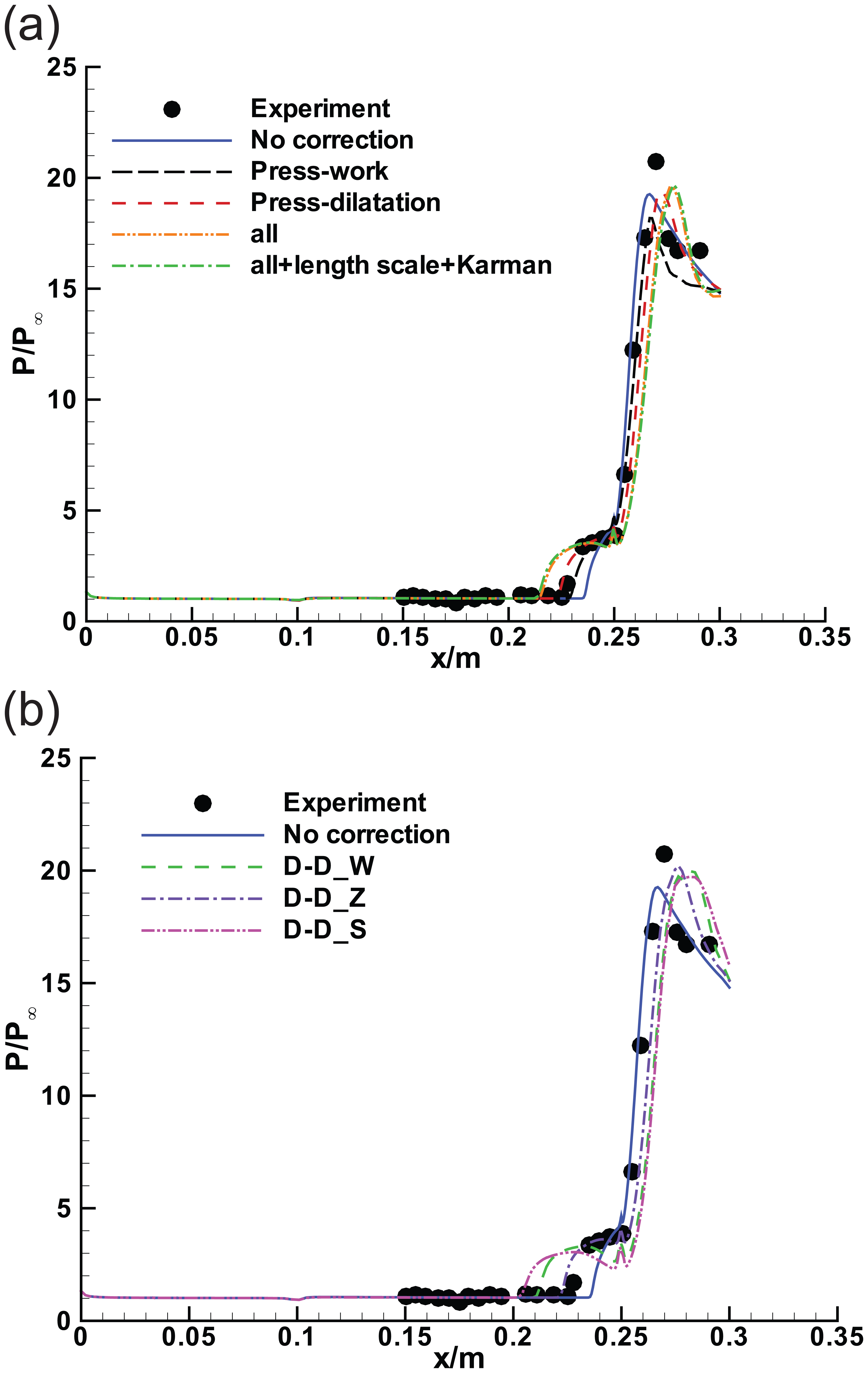
Figures 13 –17 show the calculated pressure and heat flux distributions by SST model and its compressibility corrections. The results predicted by three dilatation-dissipation models “D-D_S,”“D-D_W,” and “D-D_Z” list in one figure for easy to discern. The calculated results of SST and k-ω are given.

Figure 13.

Effect of compressibility corrections on the wall pressure by SST model for hollow cylinder-flare: (a) results of compressibility corrections except dilatation-dissipation and (b) results of three dilatation-dissipation corrections.

Figure 14.

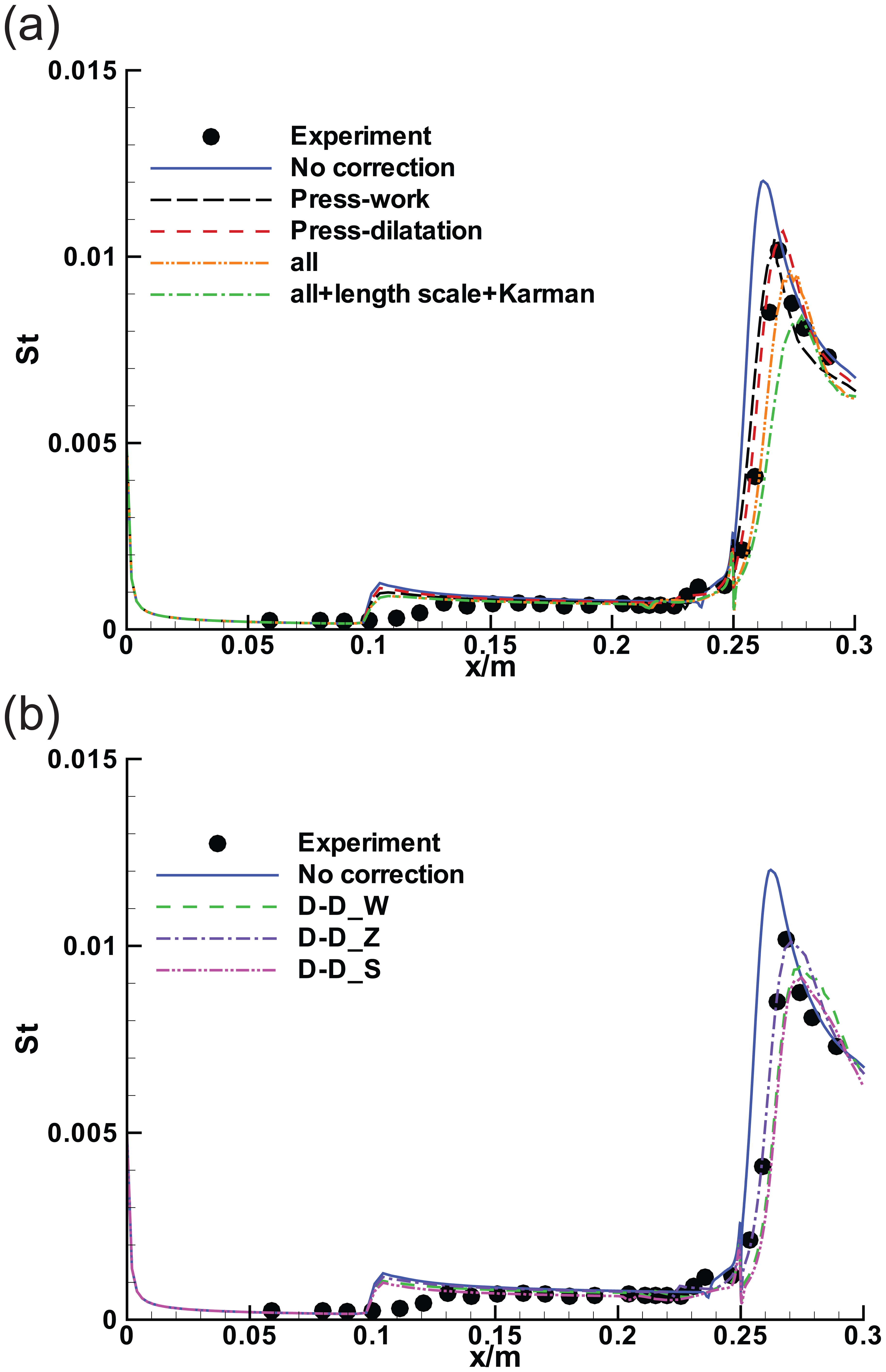
Effect of compressibility corrections on the Stanton number by SST model for hollow cylinder-flare: (a) results of compressibility corrections except dilatation-dissipation and (b) results of three dilatation-dissipation corrections.

Figure 15.

Comparison of pressure and Stanton number between SST and k-ω models for cylinder-flare at Mach 5.01: (a) wall pressure and (b) Stanton number.

Figure 16.

Effect of compressibility corrections on the wall pressure by k-ω model for hollow cylinder-flare: (a) results of compressibility corrections except dilatation-dissipation and (b) results of three dilatation-dissipation corrections.

Figure 17.

Effect of compressibility corrections on Stanton number by k-ω model for hollow cylinder-flare: (a) results of compressibility corrections except dilatation-dissipation and (b) results of three dilatation-dissipation corrections.

The results predicted by SST model is analyzed (Figures 13 and 14). The pressure distributions by original model match the experiments well and location of the separation point also agrees with the experiments. But the peak heating is higher evidently than the experiments. “Press-work” and “Press-dilatation” corrections have a little effect on pressure distribution, but it can reduce the peak heating which make results closer to the experiments. “D-D_Z” presents a slight increase in the peak value of wall pressure and an evident decrease in peak heating which make results closer to the experiments, so “D-D_Z” presents the best results. Notably, all the compressibility corrections predict an earlier separation and a later reattachment which lead to a larger separation zone than the experiments. The “Press-work,”“Press-dilatation,” and “D-D_Z” have a little influence on the separation region. But for the “D-D_S” and “D-D_W,”“all” and “all + length scale + Karman” make an evident effect on separation zone and reduce the heat transfer too much. Hence, for this test case, the “Press-work,”“Press-dilatation,” and “D-D_Z” present the acceptable results, especially the results of “D-D_Z” are the best.

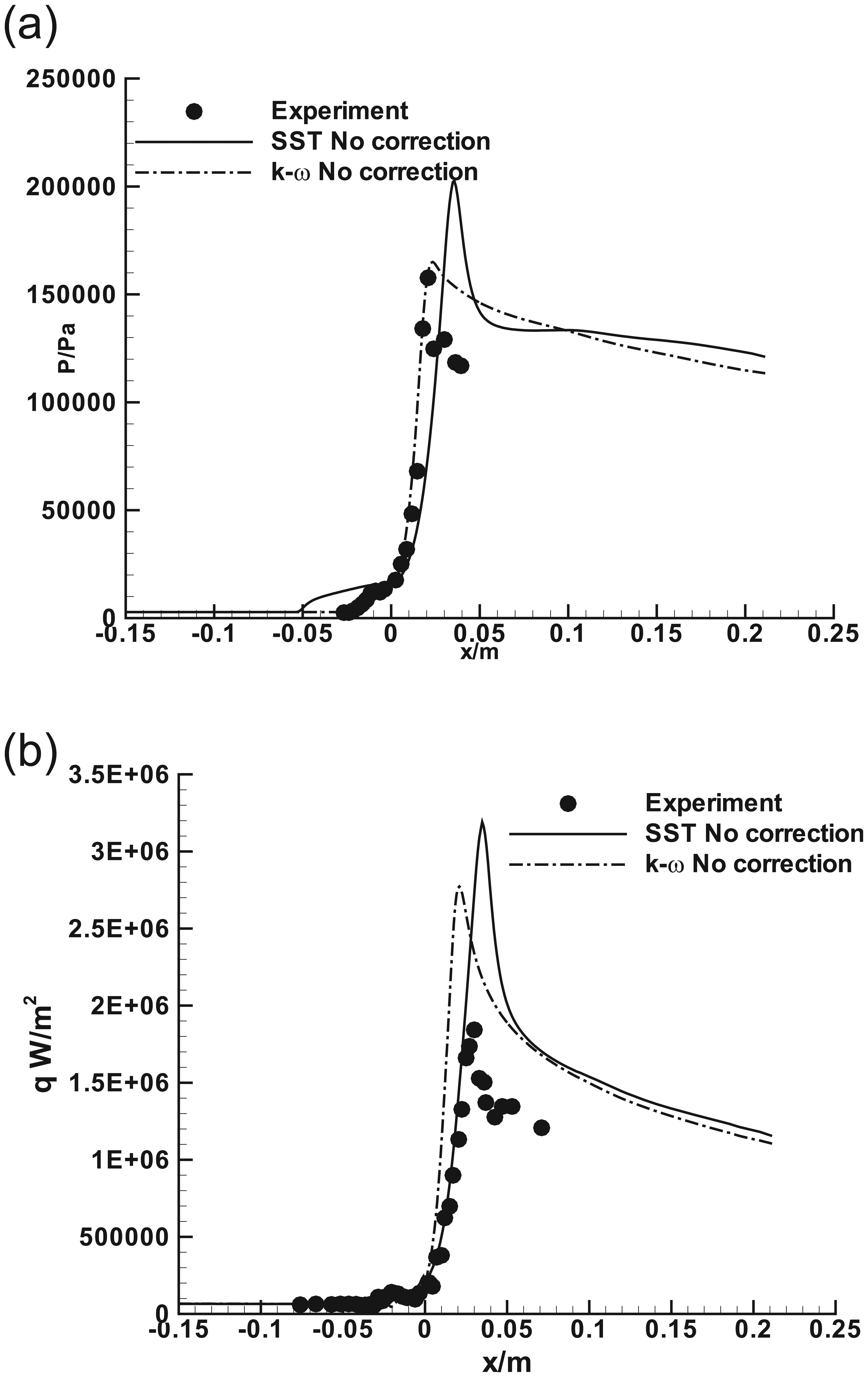
Comparison of pressure and Stanton number between original SST and k-ω models is shown in Figure 15. Boundary layer separation predicted by SST model matches experimental data well. However, the k-ω result shows that pressure rise due to the separation shock is located somewhat downstream of the experiment. The simulation with the k-ω model presents the undersized separation region. The results with both models show a slightly overestimated peak heating. The results of k-ω compressibility corrections present the similar variation trends with that of SST compressibility corrections, as shown in Figures 16 and 17.

The reason for larger separation zone predicted by compressibility corrections is analyzed. The M_T profiles of different positions x = 0.217, 0.250, and 0.258 m corresponding to attached flow, middle of separation zone, and flows near reattachment point are shown in Figure 18. It can be seen that the maximum level of M_T is approximately 0.74 in separation zone. The compressibility corrections based on M_T exhibit the large effect on the separation region. Thus, a larger derivation from the experiments is yielded. The reason is that the increasing dissipation reduces the level of TKE, then the turbulence viscosity decreases as shown in Figure 19, and the boundary layer separates earlier.

Figure 18.

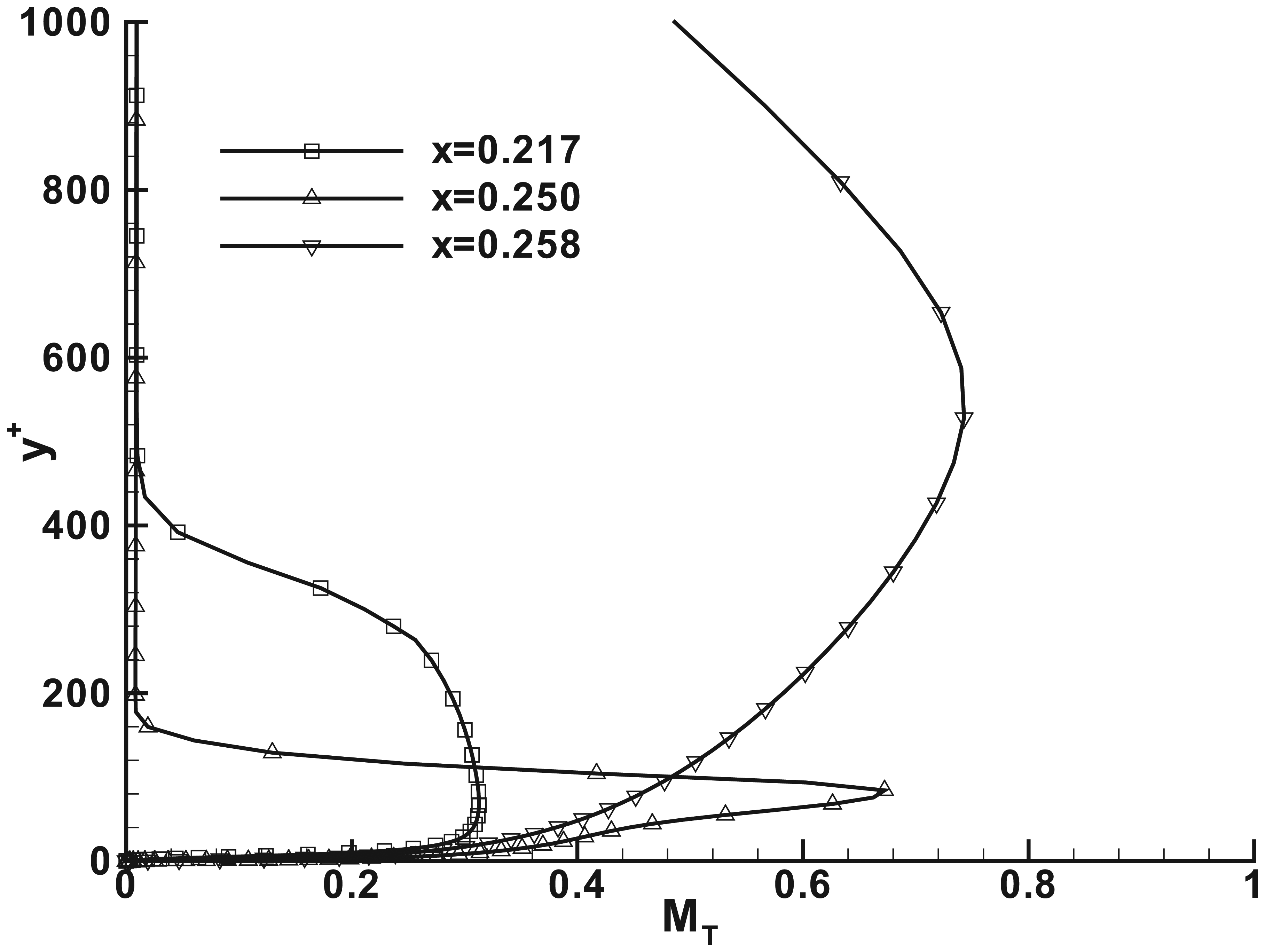
M_T profiles for hollow cylinder-flare.

Figure 19.

Turbulence eddy viscosity for cylinder-flare at Mach 5.01 by SST model and its compressibility versions.

Next, the numerical case of shock wave/boundary layer for higher Mach number is implemented. The experimental data come from Marvin et al.²⁷ The computational condition is Ma_∞ = 9.22, T_∞ = 64.5 K, ρ_∞ = 0.1367 kg/m³, and T_w = 295 K. The computation grid is shown in Figure 20 and the normal distance of first layer grid is 1 × 10⁻⁶ m.

Figure 20.

Computational grid for compression corner.

Figure 21 gives the wall pressure and heat transfer distributions predicted by original SST and k-ω models. Experimental data are also presented for comparison. The SST simulation yields an earlier separation than the k-ω model. Separation zone size is larger than the experiments. However, separation zone predicted by k-ω model is more consistent with the experiments. The peak heating is overpredicted by both turbulence models, even though the reattachment points agree well with the experiments.

Figure 21.

Comparison of pressure and heat flux between SST and k-ω models: (a) wall pressure and (b) heat transfer.

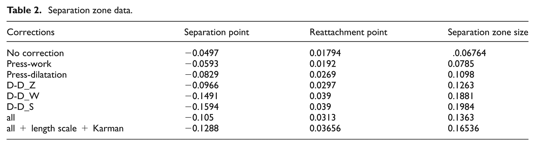
Figure 22 shows the pressure distributions by seven compressibility corrections for SST models. It can be seen that all the compressibility corrections make the separation region larger. The wall pressure curves shift right because of earlier separation points and delayed reattachment points. But the corrections have little effect on peak pressure. In this test case, all the compressibility corrections (including “Press-work,”“Press-dilatation,” and “D-D_Z”) exhibit an obvious deviation for the simulation of separation region. Table 2 gives the detailed data for the positions of separation points, reattachment points, and separation zone size. The results show that the “Press-work” correction has the smallest effect on separation zone, the effect of “Press-dilatation” is slightly larger, and dilatation-dissipation has the largest effect. Among all the dilatation-dissipation corrections, correction level of “D-D_Z” is the least.

Figure 22.

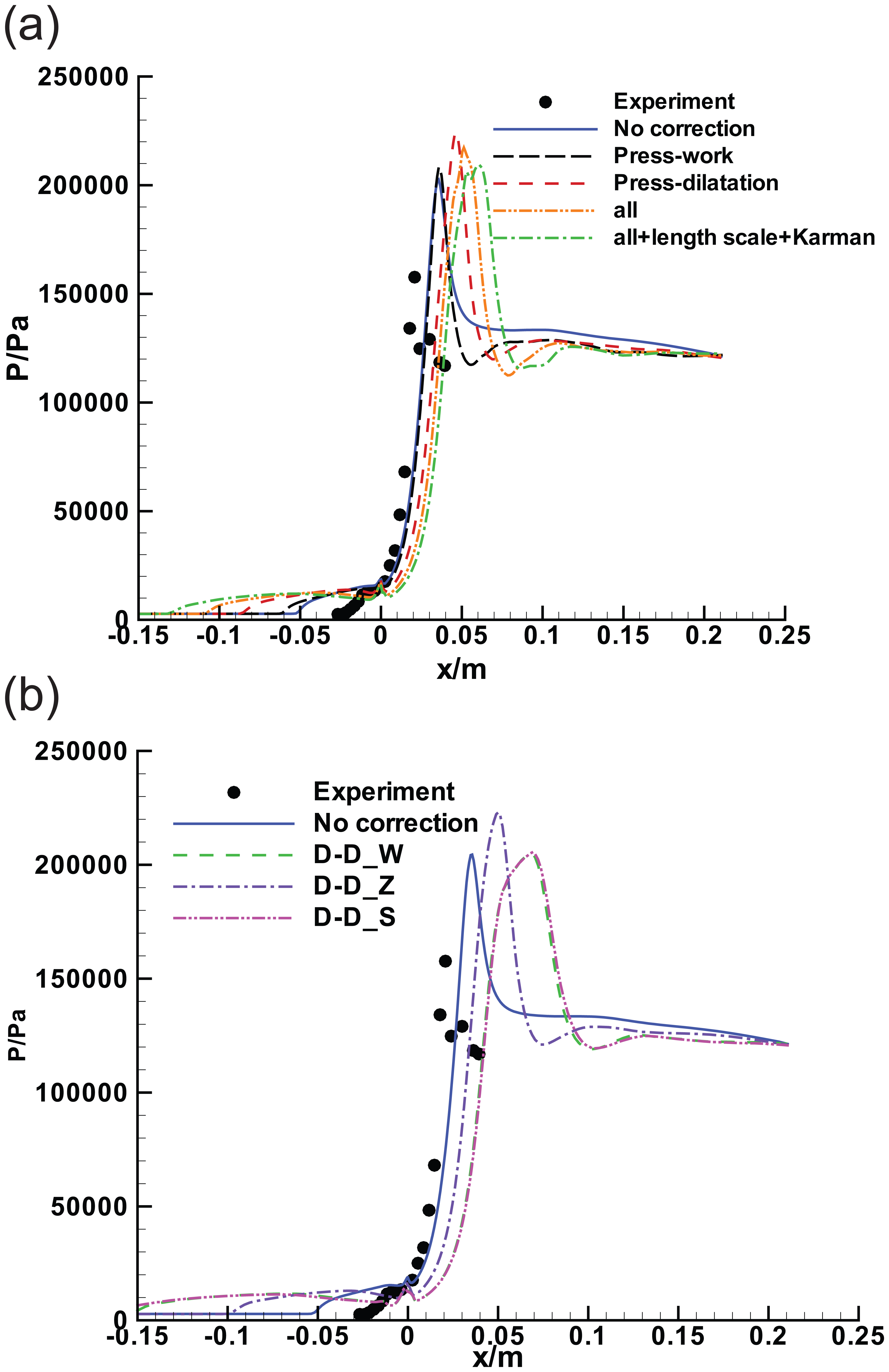
Effects of compressibility corrections on the wall pressure by SST model for compression corner: (a) results of compressibility corrections except dilatation-dissipation and (b) results of three dilatation-dissipation corrections.

Table 2.

Separation zone data.

Corrections	Separation point	Reattachment point	Separation zone size
No correction	−0.0497	0.01794	.0.06764
Press-work	−0.0593	0.0192	0.0785
Press-dilatation	−0.0829	0.0269	0.1098
D-D_Z	−0.0966	0.0297	0.1263
D-D_W	−0.1491	0.039	0.1881
D-D_S	−0.1594	0.039	0.1984
all	−0.105	0.0313	0.1363
all + length scale + Karman	−0.1288	0.03656	0.16536

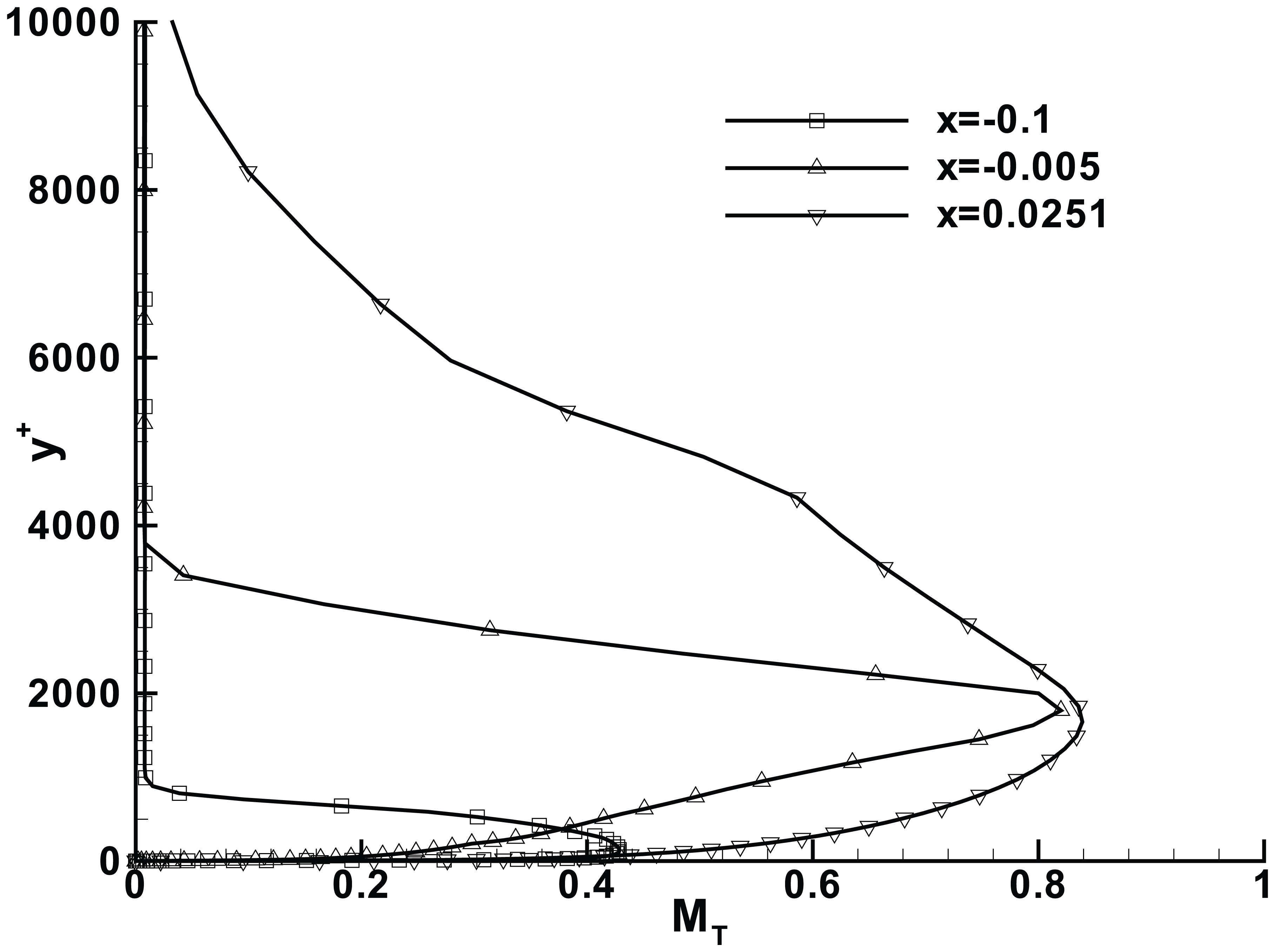
The M_T curves of three different positions x = −0.1, −0.005, and 0.0251 m which located in attached flow, separation zone, and region near reattachment point for original SST model are given in Figure 23. The maximum M_T is about 0.82. It indicates that the compressibility corrections based on M_T exhibit the great influence on separation zone which lead to a larger separation as shown in Figure 22. The compressibility corrections on the separation zone produce a deviation from the experiments which is similar to the results of cylinder-flare test case at Mach 5.01.

Figure 23.

M_T profiles for compression corner at Mach 9.22.

Figure 24 gives the Stanton number distribution predicted by compressibility corrections. The trend of larger separation region can also be observed. Besides, the peak value is still higher than experimental data, although the compressibility corrections can reduce the peak heating. As shown in Figure 24, “Press-work” can reduce peak heating very little, “press-dilatation” takes second place, and dilatation-dissipation has the greatest effect on peak heating. “all + length scale + Karman” method can reduce peak heating further. “all + length scale + Karman” predicts the peak heating close to the experiments, but the separation point and reattachment point have a large deviation from the experimental data. Therefore, this consistence should be a coincidence.

Figure 24.

Effects of compressibility corrections on Stanton number by SST model for compression corner: (a) results of compressibility corrections except dilatation-dissipation and (b) results of three dilatation-dissipation corrections.

The magnitudes of production, dissipation, and compressible terms normalized by $ρ V_{\infty}^{3} / L$ are presented in Figure 25. Each term of compressibility corrections for “all + length scale + Karman” located at unseparated position x = −0.2 m is given in Figure 25. The production and incompressible dissipation term ε_s are also given for comparison. It can be seen that the peak value of production term is generated at y⁺ = O(10) which is similar to that of zero pressure gradient flat plate boundary layer. The pressure-dilatation term can be observed noticeably and others are very small.

Figure 25.

Contributions of compressibility correction terms to TKE as a function of y⁺ at x = −0.2 m for compression corner at Mach 9.22.

Figure 26 gives the contributions of compressibility correction terms to TKE as a function of y⁺ near peak heating. Besides the peak near wall region y⁺ = O(10), a new peak of TKE production occurs at y⁺ about 1000. However, the peak of TKE production for original model only occurs at y⁺ = O(10) which explains why original model predicts an overshoot of the peak heating. The pressure work, pressure-dilatation, and dilatation-dissipation terms cannot be ignored. In order to analyze the effects of the reattachment shock amplifying mechanism at the peak heating location, Figure 27 gives plot of TKE distribution as a function of streamwise direction x at y⁺ = 1000. The figure shows that the pressure work has the positive value at peak heating location which helps to increase the TKE while the pressuer-dilatation and dilatation-dissipation have negative value resulting in the decrease of TKE.

Figure 26.

Contributions of compressibility correction terms to TKE as a function of y⁺ near peak heating location for compression corner at Mach 9.22: (a) results by original SST model and (b) results by compressibility correction.

Figure 27.

Contributions of compressibility correction terms to TKE versus x at y⁺ = 1000 for compression corner at Mach 9.22.

Figures 28 and 29 give the results of compressibility corrections for k-ω model. The variation trend by k-ω model is consistent with the SST results. Similarly, the separation zone becomes larger detrimentally and the peak heating is far from the experiments. Because the separation zone itself is smaller predicted by original k-ω model, the separation zone predicted by corrected k-ω model is better than SST.

Figure 28.

Effect of compressibility corrections on wall pressure by k-ω model for compression corner at Mach 9.22: (a) results of compressibility corrections except dilatation-dissipation and (b) results of three dilatation-dissipation corrections.

Figure 29.

Effects of compressibility corrections on heat flux by k-ω model for compression corner at Mach 9.22: (a) results of compressibility corrections except dilatation-dissipation and (b) results of three dilatation-dissipation corrections.

Finally, the test case of shock wave/boundary layer flow for higher Mach number is performed in order to validate the above conclusions. The compression corner²⁷ of flow conditions M_∞ = 11.3, T_∞ = 61 K, ρ_∞ = 0.08246 kg/m³, and T_w = 300 K is simulated numerically. The results of SST and k-ω models are shown in Figures 30 –33. It can be seen that the capture of separation point is relatively accurate, especially for k-ω model. But the peaks of pressure and heat flux are overestimated compared with the experiments. The separation and reattachment points by compressibility corrections are largely deviated from the experiments and the separation zone is larger with the increasing Mach numbers. The compressibility corrections cannot enhance the simulation accuracy of the peak pressure and heating and are still far from the experiments. The influence trend is similar to the above test cases which verified the above conclusions further. The plot of turbulence Mach number as a function of y⁺ is shown in Figure 34, and similarly curves of three locations before separation, interior to separation zone, and near reattachment point are given. The maximum M_T is about 0.93 which explains the reason for larger separation zone.

Figure 30.

Effect of compressibility corrections on wall pressure by SST model for compression corner at Mach 11.3: (a) results of compressibility corrections except dilatation-dissipation and (b) results of three dilatation-dissipation corrections.

Figure 31.

Effect of compressibility corrections on heat flux by SST model for compression corner at Mach 11.3: (a) results of compressibility corrections except dilatation-dissipation and (b) results of three dilatation-dissipation corrections.

Figure 32.

Effects of compressibility corrections on wall pressure by k-ω model for compression corner at Mach 11.3: (a) results of compressibility corrections except dilatation-dissipation and (b) results of three dilatation-dissipation corrections.

Figure 33.

Effects of compressibility corrections on heat flux by k-ω model for compression corner at Mach 11.3: (a) results of compressibility corrections except dilatation-dissipation and (b) results of three dilatation-dissipation corrections.

Figure 34.

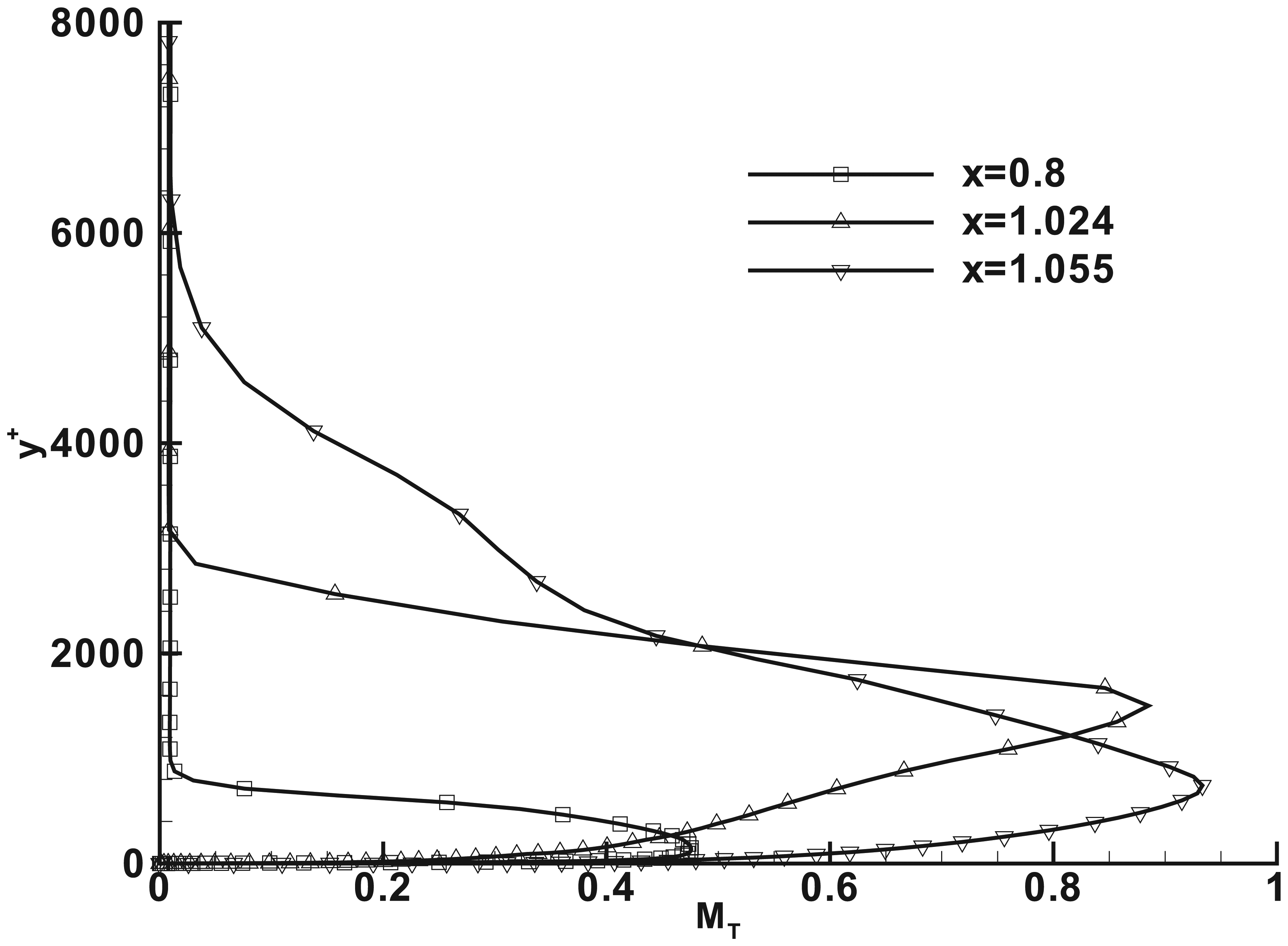
M_T profiles as a function for compression corner at Mach 11.3.

The physical mechanism of shock wave/boundary layer interaction is different from that of the flat plate boundary layer. First, in DNS results of He,³¹ the effect of adverse pressure gradient on compressible turbulent boundary layer is that a second peak of the turbulent production occurs in the outer layer. However, the TKE reaches a peak near the wall for flat plate of zero adverse pressure gradients. Thus, the balance mechanism consists of production, dissipation, pressure-dilatation, and dilatation-dissipation.

Secondly, because of adverse pressure gradient and viscous effect, the separation occurs for compression corner. The compressibility correction models constructed by turbulence Mach number exhibit compressible effect on turbulent structures with the increase of turbulence Mach number. However, the increase of turbulence Mach number in separation zone is not caused by the increasing compressible effect. In contrast, the compressible effect should be weaker due to the decrease of flow velocity in separation zone. Therefore, it is unreasonable physically that compressibility correction models based on turbulence Mach number take effect in separation zone. The compressibility corrections make the separation zone larger and generate more deviation from experimental data. Therefore, the effect of compressibility corrections on separation zone is detrimental.

Rapid compression fix

In order to assess the suitability of rapid compression fix method, numerical simulation for compression corner at Mach number 11.3 is carried out.⁸ The results in Figure 35 show that the predicted separation zone by SST and k-ω turbulence models with compressibility corrections is larger than that by original model. It can be seen that the k-ω simulations present the largest separation region. Although the peak heating can be reduced to a value slightly lower than experiments, the deviation of separation and reattachment points from experiments is larger.

Figure 35.

Wall pressure and heat flux computed by rapid compression fix versions for SST and k-ω models: (a) wall pressure and (b) heat transfer.

Density-corrected model by Catris and Aupoix

In order to evaluate the suitability of density-corrected model proposed by Catris and Aupoix,¹⁹ the test cases of compression corners at Mach 9.22 and 11.3 are numerically simulated. Comparisons of wall pressure between experimental data and calculated results by original k-ω and density-corrected model are shown in Figure 36(a). It can be known that the density-corrected model does not have strong influence on pressure prediction. The peak value of pressure is not sensitive to the density-corrected model. However, the modified turbulence model is superior to original turbulence model in the prediction of the peak value of heat flux. Comparisons of heat flux between experimental data and calculated results by original and density-corrected models are shown in Figure 36(b). It can be seen that the heat flux is overestimated seriously by the original model while the result of density-corrected model accords well with experimental data. The curves of pressure and heat flux indicate that the density-corrected model has a little influence on the size of separation region and maintain the accurate prediction on separation by original turbulence model. Figure 37 shows similar variation trend for M_∞ = 11.3. The results have shown that the simulation by density-corrected model in this article is superior to the above compressibility corrections.

Figure 36.

Wall pressure and heat flux computed by density-corrected model at Mach 9.22: (a) wall pressure and (b) heat transfer.

Figure 37.

Wall pressure and heat flux computed by density-corrected model at Mach 11.3: (a) wall pressure and (b) heat transfer.

Real gas effects

In this chapter, when freestream Mach number is greater than 10, the total temperature for the flat plate case at Mach 11.1 and compression corner case at Mach 11.3 are 1641 and 1619 k, respectively. Therefore, taking the excitation of vibrational energy into account, the specific heat is not constant. The specific heat variations with the temperature are considered. The results in Figures 38 and 39 show that there are almost no visible differences between the results of constant and variable specific heat.

Figure 38.

Effects of specific heat variations on friction coefficient and heat flux for the flat plate case at Mach 11.1: (a) friction coefficient and (b) heat flux.

Figure 39.

Effects of specific heat variations on pressure and heat flux for the compression corner at Mach 11.3: (a) wall pressure and (b) heat flux.

Conclusion

In this article, the application study of the various compressibility corrections including pressure work, pressure-dilatation, dilatation-dissipation (Sarkar, Zeman, and Wilcox) and synthetical correction models are performed for hypersonic boundary layer flows. The two typical problems of flat plate boundary layer and shock wave/boundary layer interaction are calculated with Favre averaged Navier–Stokes equations. SST and k-ω turbulence model and their correction version are employed. The results of wall pressure, Stanton number, and friction distributions are compared with experiments.

The following conclusions can be drawn for the hypersonic flat plate turbulent boundary layer flows:

The original k-ω SST can get the results in agreement well with the experiments at Mach number 5–8. However, the heat flux is overpredicted when Mach number is about 10 The compressibility corrections can reduce the friction coefficients and heat flux.

In terms of the influence of compressibility corrections on calculated results, the pressure work and pressure-dilatation present results in the range of experimental data at low Mach number and improves the heat flux results at high Mach number. For three dilatation-dissipation models, results of Sarkar and Wilcox have the large derivation from the experiments, but Zeman model can achieve acceptable results. Hence, Zeman model is prior to be chosen among the three dilatation-dissipation models.

The following conclusion can be drawn from the studies for shock wave/boundary layer interaction:

The compressibility corrections make the separation point move upstream and reattachment point shift downstream; thus a larger separation zone is generated. The reason for larger separation zone predicted by compressibility corrections is that the increase of the M_T in separation zone caused by the increasing TKE leads to a decrease in Reynolds stress. However, the increase of the M_T in separation zone is not caused by compressibility effects. Therefore, we think that the compressibility corrections that take effect in separation zone are unreasonable.

Although the prediction of separation point by original k-ω SST is relatively accurate, especially for k-ω model, the peaks of pressure and heat flux are overestimated. However, compressibility corrections generate the larger deviation of separation and reattachment points from the experiments. The pressure work correction has the least effect on results, the effect of pressure-dilatation is slightly larger, and dilatation-dissipation has the largest effect. The effect tendency of the three dilation-dissipation corrections is the same with that in plate boundary layer. “Sarkar” creates the largest difference, “Wilcox” takes second place, and “Zeman” generates the smallest. The deviation becomes larger with the increasing Mach number. The simulation accuracy of pressure and heat flux peaks does not improve by compressibility corrections.

Rapid compression fix method makes separation zone larger and heat transfer lower by adding dissipation. But its predicted reattachment point has much deviation.

The peak heating predicted by density-corrected model matches the experimental data well at the cost of a little larger separation zone. The overestimation of heat flux near the reattachment point in shock wave/boundary layer interaction simulation is improved by density-corrected model. The density-corrected model enhances the prediction accuracy of shock wave/boundary layer interaction simulation effectively.

Footnotes

Academic Editor: Moran Wang

Declaration of conflicting interests

The author(s) declared no potential conflicts of interest with respect to the research, authorship, and/or publication of this article.

Funding

The author(s) disclosed receipt of the following financial support for the research, authorship, and/or publication of this article: This work was supported by Aeronautics Science Foundation of China (20141251015).

References

Favre

The mechanics of turbulence. New York: Gordon and Breach, 1962, pp.367–380.

Wilcox

DC.

Turbulence modeling for CFD. 3rd ed. La Cañada Flintridge, CA: DCW Industries, Inc., 2006, pp.243–261.

Sarkar

Erlebacher

Hussaini

. The analysis and modeling of dilatational terms in compressible turbulence. NASA-CR-181959, 1 December 1989. Hampton, VA: NASA Langley Research Center.

Wilcox

DC.

Dilatation-dissipation corrections for advanced turbulence models. AIAA J 1992; 30: 2639–2646.

Zeman

Dilatational dissipation: the concept and application in modeling compressible mixing layers. Phys Fluids A: Fluid 1990; 2: 178–188.

Sarkar

The pressure-dilatation correlation in compressible flows. Phys Fluids A: Fluid 1992; 4: 2674–2682.

Speziale

Sarkar

. A preliminary compressible second-order closure model for high speed flows. NASA-CR-181875, July 1989. Hampton, VA: NASA Langley Research Center.

Coakley

Huang

. Turbulence modeling for high speed flows. In: Proceedings of the 30th aerospace sciences meeting and exhibit, Reno, NV, 6–9 January 1992, paper no. AIAA-92-0436. Reston, VA: AIAA.

Vuong

Coakley

. Modeling of turbulence for hypersonic flows with and without separation. In: Proceedings of the 25th AIAA aerospace sciences meeting, Reno, NV, 12–15 January 1987, paper no. AIAA-87-0286. Reston, VA: AIAA.

10.

Coakley

. Turbulence modeling methods for the compressible Navier-Stokes equations. In: Proceedings of the 16th fluid and plasma dynamics conference, Danvers, MA, 12–14 July 1983, paper no. AIAA-83-1693. Reston, VA: AIAA.

11.

Sarkar

The stabilizing effect of compressibility in turbulent shear flow. J Fluid Mech 1995; 282: 163–186.

12.

Sinha

Balasridhar

Conservative formulation of the k-ε turbulence model for shock–turbulence interaction. AIAA J 2013; 51: 1872–1882.

13.

Grasso

Falconi

High-speed turbulence modeling of shock-wave/boundary-layer interaction. AIAA J 1993; 31: 1199–1206.

14.

Rumsey

CL.

Compressibility considerations for k-ω turbulence models in hypersonic boundary-layer applications. J Spacecraft Rockets 2010; 47: 11–20.

15.

Deng

Mao

ML.

Assessment of two turbulence models and some compressibility corrections for hypersonic compression corners by high-order difference schemes. Chinese J Aeronaut 2012; 25: 25–32.

16.

Liu

JY.

Compressibility correction for the SST two-eq22 turbulence model in hypersonic flows. J Astronaut 2012; 33: 1719–1726 (in Chinese).

17.

Dong

Zhou

The improvement of turbulence modeling for the aerothermal computation of hypersonic turbulent boundary layers. Sci China Phys Mech Astron 2010; 53: 369–379.

18.

X-l

D-x

Y-w.

Assessment of the compressible turbulence model by using the DNS data. Chin J Theor Appl Mech 2012; 44: 222–229.

19.

Catris

Aupoix

Density corrections for turbulence models. Aerosp Sci Technol 2000; 4: 1–11.

20.

Gao

Jiang

Lee

CH.

Improvement and application of wall function boundary condition for high-speed compressible flows. Sci China Technol Sci 2013; 56: 2501–2515.

21.

Gao

Lee

CH.

A numerical study of turbulent combustion characteristics in a combustion chamber of a scramjet engine. Sci China Technol Sci 2010; 53: 2111–2121.

22.

Kim

Rho

OH.

An improvement of AUSM schemes by introducing the pressure-based weight functions. Comput Fluids 1998; 27: 311–346.

23.

van Leer

. Towards the ultimate conservative difference scheme V. A second order sequel to Godunov’s method. J Comput Phys 1979; 32: 101–136.

24.

Yoon

Jameson

. Lower-upper symmetric Gauss-Sediel method for the Euler and Navier-Stoker equations. AIAA J 1988; 26: 1025–1026.

25.

Menter

. Zonal two equation k-ω turbulence models for aerodynamic flows. In: Proceedings of the 23rd fluid dynamics, plasma dynamics, and lasers conference, Orlando, FL, 6–9 July 1993, paper no. AIAA-1993-2906. Reston, VA: AIAA.

26.

Holden

MS.

An experimental investigation of turbulent boundary layers at high mach number a Reynolds numbers. NASA-CR-112147, 1 November 1972. Hampton, VA: NASA Langley Research Center.

27.

Marvin

Brown

Gnoffo

JG.

Experimental database with baseline CFD solutions: 2-D and axisymmetric hypersonic shock-wave/turbulent-boundary-layer interactions. NASA TM-2013-216604, 1 November 2013. Hampton, VA: NASA Langley Research Center.

28.

Van Driest

. Problem of aerodynamic heating. Aeronaut Eng Rev 1956; 15: 26–41.

29.

Van Driest

. Turbulent boundary layer in compressible fluids. J Aeronaut Sci 1951; 18: 145–160.

30.

Paciorri

Dieudonné

Degrez

. Validation of the Spalart-Allmaras turbulence model for application in hypersonic flows. In: Proceedings of the 28th fluid dynamics conference, Snowmass Village, CO, 29 June–2 July 1997, paper no. AIAA-97-2023. Reston, VA: AIAA.

31.

High order methods and numerical simulations of shock wave/turbulent boundary layer interaction problems. Beijing, China: University of Chinese Academy of Sciences, 2013.

Investigation of turbulence models with compressibility corrections for hypersonic boundary flows

Abstract

Keywords

Introduction

Numerical methods

Governing equations

Compressible form of two-equation turbulence models

Pressure work and pressure-dilatation corrections

Dilatation-dissipation correction

Synthetical correction

Turbulence length scale correction

Rapid compression fix

Catris and Aupoix correction

Results and discussions

Compressibility corrections

Hypersonic flat plate boundary layer

Shock wave/boundary layer interaction

Rapid compression fix

Density-corrected model by Catris and Aupoix

Real gas effects

Conclusion

Footnotes

Declaration of conflicting interests

Funding

References