
Abstract
Accurately predicting short-term transport demand for an individual logistics company involved in a competitive market is critical to make short-term operation decisions. This article proposes a combined grey–periodic extension model with remnant correction to forecast the short-term inter-urban transport demand of a logistics company involved in a nationwide competitive market, showing changes in trend and seasonal fluctuations with irregular periods different to the macroeconomic cycle. A basic grey–periodic extension model of an additive pattern, namely, the main combination model, is first constructed to fit the changing trends and the featured seasonal fluctuation periods. In order to improve prediction accuracy and model adaptability, the grey model is repeatedly modelled to fit the remnant tail time series of the main combination model until prediction accuracy is satisfied. The modelling approach is applied to a logistics company engaged in a nationwide less-than-truckload road transportation business in China. The results demonstrate that the proposed modelling approach produces good forecasting results and goodness of fit, also showing good model adaptability to the analysed object in a changing macro environment. This fact makes this modelling approach an option to analyse the short-term transportation demand of an individual logistics company.
Keywords
Introduction
The main business of transport-oriented logistics companies is freight transport. Accurately predicting transport demand is very important for these logistics companies to arrange transportation tasks, optimise resource allocation and reduce the operating cost of production. Especially for large-scale transportation logistics companies engaged in nationwide business, accurately predicting short-term inter-urban transport demand can help to optimise transport plans and vehicle scheduling and improve profitability. 1 At present, the logistics industry in China is in an upgrading period of integration; a few large logistics enterprises have been growing. However, the efficiency of resource integration and utilisation needs to be improved. This article mainly focuses on short-term inter-urban transport demand forecasting for large transport-oriented logistics companies, providing support to short-term operation decision-making.
West et al. 2 acknowledge that the uncertainty, randomness and fuzziness of freight transport demand leads to complexity when forecasting. Freight transport demand forecasting methods can be divided into qualitative and quantitative forecasting, according to Zhou and Dai. 3 Qualitative forecasting mainly uses the personal experience and subjective judgement ability of professionals or decision-makers to find out the law and to make judgements about the future. This forecasting method is simple, but subjective and one sided. Its prediction accuracy is also not high. The qualitative forecasting methods used in freight transport demand forecasting mainly include personal judgement, the Delphi technique and the subjective probability method, which are usually used as supplementary decision-making tools. Quantitative forecasting methods use a variety of mathematical models to predict future development based on historical statistical data and relevant information. Commonly used methods for quantitatively predicting transport demand include time series analysis, regression analysis, the transport coefficient method, the velocity ratio method and the neural network prediction method.4–9
The quantitative prediction process includes model selection, model calculation and result adjustment. 10 The first step is to select a model or a model combination according to the characteristics of the object to be forecast and the decision-making purpose. The second step is to carry out data collection and model calculation. The third step is to analyse the reliability and validity of the results and to carry out model adjustment if needed. In the literature, forecasting macro national transportation demand or regional long-term comprehensive transportation demand has been mostly studied.11–13 Single models are mostly used, and a few combined models are seen. Most of the prediction results show that the factors influencing macro and long-term freight transport demand are relatively clear, the trend and periods of which are closely related to the trend and periods of national and regional economic development. This kind of prediction is not sufficient to support the microscopic operation management of a firm or company, however, because the short-term freight transportation demand of a firm or company suffers from more uncertain influencing factors. The freight transport demand of a firm or company is related not only to the influencing factors of macro transportation demand but also to the micro influencing factors such as market position, marketing strategy and customer relationships. McCarthy 14 and Lee et al. 15 acknowledge that these two kinds of factors are continually changing, and the connections between them are difficult to accurately express, showing a kind of grey system relation. Fang et al. 16 argued that to some extent, the micro transportation demand of a firm or company will rise and fall along with macroeconomic fluctuations, but its fluctuation period and development trend are often unclear and fuzzy.
The grey model GM(1,1) and its improved models have been successfully applied to forecast long-term and short-term transportation demands and have shown promising results. In fact, grey models do not require data as strictly as other regression models and have good adaptability to short-term and data-limited predictions. In terms of processing the seasonal fluctuations and trends of a transportation demand time series with a fixed period, it has been suggested to separate the time series by smoothing the data into a trend component, fluctuation component and error component and then using different models to fit the period and the trend, respectively, and combine them, according to Barrow. 17 This method was successfully applied to forecast the transport demand of a small logistics company (an export container transportation business near the port area) developed by Fang et al. 16 Seasonal Autoregressive Integrated Moving Average (SARIMA) model is another forecasting method usually used to analyse non-stationary time series with trend and seasonality. 18 However, when the seasonal fluctuation period is not very stable or clear, this method may confuse the subsequent analysis. At this time, the data series needs to be further modelled to find the trend and periods. A Fourier series indicates that any time series function can be seen as the superposition of infinite vibration waves with different frequencies. 19 Brockwell and Davis 20 stated that power spectrum analysis and periodic extension are the two most effective methods to identify and extract the dominant periods of a time series.
For a time series with trend and periodic waves, it can neither reveal the periodic feature very well by only using grey system models nor can it reveal the trend by only using periodic extension models (PEMs). The approach proposed by Fang et al. 16 can cope with the effect of macroeconomic fluctuation on small-sized enterprises. However, data pre-processing eliminates the irregular data, which helps to improve the stability of the observed data series. In this article, the sample logistics company’s business data have the dual characteristics of trend and non-fixed periods, which result from the additive fluctuations of macro and micro factors. Liu and Lin 21 indicated that trying a combination model of the grey model and PEM gives a way to solve this problem.
The objective of this study is to construct a combined grey-PEM with remnant correction to cope with short-term and data-limited prediction problem with trend and non-stationary periods, which is characterised by the sample business data from a real logistics company. The context of the model is characterised by one distinct element: the short time series with trend and non-stationary periods. In the modelling process, the main combination model is constructed by superposing a grey model GM(1,1) with a PEM, in which GM(1,1) is chosen to fit the trend, and the PEM is constructed to capture the featured seasonal fluctuation periods. In order to improve prediction accuracy and model adaptability, remnant correction is carried out by fitting the remnant tail time series of the main combination model until the prediction accuracy is satisfied.
The rest of this article is organised as follows: In the following section, a detailed modelling process and the model architecture are presented. This is followed by model application, including data description, modelling results, forecasting performance and model comparison. Conclusions and implications are then drawn.
Modelling
The basic idea of building a GM(1,1)-periodic extension model with remnant correction (RC-GMPEM) is to make full use of the trend characteristics of exponential growth in the GM(1,1) model to improve the predicting accuracy. 21 While taking into account the seasonal fluctuations in the time series, the PEM is used to identify precisely the seasonal fluctuation period of the observed time series and carry out the forecasting revision in the observed fluctuant points; then, the trend component and seasonal component are superposed using the additive modelling of the seasonal time series in order to obtain the main combination model. 17
The modelling process of RC-GMPEM is illustrated in Figure 1. The modelling process can be divided into five steps. The first step is to test the smoothness and quasi-exponential of the original time series. Passing the test of the quasi-exponential is the premise to establish the GM(1,1) model. The second step is to build the GM(1,1) model of the time series according to the modelling method of grey system theory, if the time series has passed the test and fits the trend components of the time series. In the third step, the PEM is built to identify the fluctuation period of the time series; this needs to correct the peak points of the large fitting errors caused by seasonal fluctuations. The fourth step is to combine the GM(1,1) model with the PEM to obtain the main combination model (GMPEM) according to the additive modelling idea of the seasonal time series and then test the prediction accuracy of the main combination model. In the fifth step, GM(1,1) is repeatedly modelled to fit the remnant tail series of the main combination model until the prediction accuracy is satisfied in the fourth step and then we have the final RC-GMPEM. We describe the detailed modelling steps in the following subsections.

Modelling process of the RC-GMPEM.
Test the smoothness and quasi-exponential of the time series
Assuming that
Test the smoothness of
The smoothness of the series can be measured by the smoothness ratio

When the
where
Taking a proper constant c, and making
Test the quasi-exponential of
Generally, the randomness of the original time series may be reduced after repeated AGO, and the generated series will show the law of exponential growth according to Benítez et al.
23
At the same time, Kayacan et al.
24
stated that, if the r-AGO series of
For
Because
Build the GM(1,1) model for the generated transport demand series
By building the differential equation of the GM(1,1) model of the generated series
The GM(1,1) differential equation of

where a and b are the waiting-estimated parameters.
At the moment k, when the time interval

When

Assuming that

Let

where a and b are the waiting-estimated parameters.
Assuming that

then equation (6) is equivalent to

Then, we can obtain the expression of the waiting-estimated parameters a and b

According to equation (4), by solving the differential equation, we obtain

The discrete form is

Let
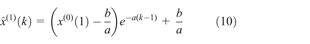
Let

Equation (11) is the response function of the 1-AGO series of the GM(1,1) of the inter-urban transport demand time series.
Thus, according to

Build the PEM model for the generated transport demand series
In order to overcome the shortcoming that the GM(1,1) model is not excellent at fitting seasonal fluctuations, we can build the PEM of the remnant series, which is constituted by the predicted values and observed values of the GM(1,1) model. Through this, we can extract the dominant period by discerning the periodic fluctuation phenomena of the remnant series and then modify the predicted values on the inflection point of periodic variation. The modelling steps are as follows:
Build the remnant series
Build the mean generating function of the remnant series
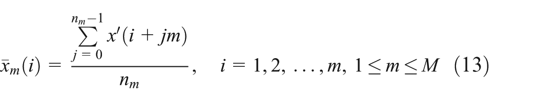
In equation (13), n is the length of the remnant series
Through these calculations, we can obtain the mean generating function matrix of

We now make the periodic extension the mean generating function

In equation (15),
3. Extract the dominant period m. According to variance analysis theory, we can use equation (16) to test whether the series
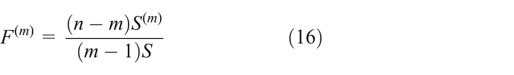
where
For a given confidence level
4. Extract the other dominant periods. We generate a new series

By repeating steps (2) and (3) for the new series
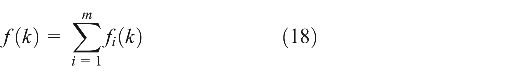
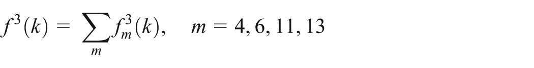
5. Superposition. Superpose the values of different periods at the same time and write it as
Build the main combination model (GMPEM)
According to the additive modelling idea of seasonal time series, we make

Test the prediction accuracy of the GMPEM
The prediction accuracy of the GMPEM can be measured by variance ratio c and small error probability p. 21 The calculations are as follows

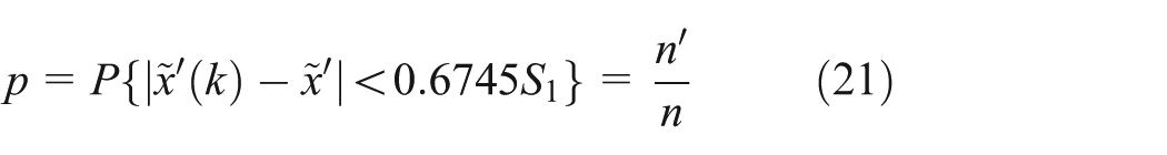
where
The prediction accuracy can be quantified into different levels according to the values of c and p (see Table 1). If the values of c and p are not at the same level, we take the greater value to be the prediction accuracy level of the model.
Prediction accuracy level measured by c and p.

Source: Liu and Lin. 21
Correct the random error of the GMPEM by remnant correction
In order to reduce the influence of random error of the GMPEM on the prediction accuracy, we build the GM(1,1) model of the remnants of the combination model to correct the random error, so that we can improve the precision of the prediction accuracy further.
Assuming that

Therefore, we can obtain the remnant series of the GMPEM, namely,

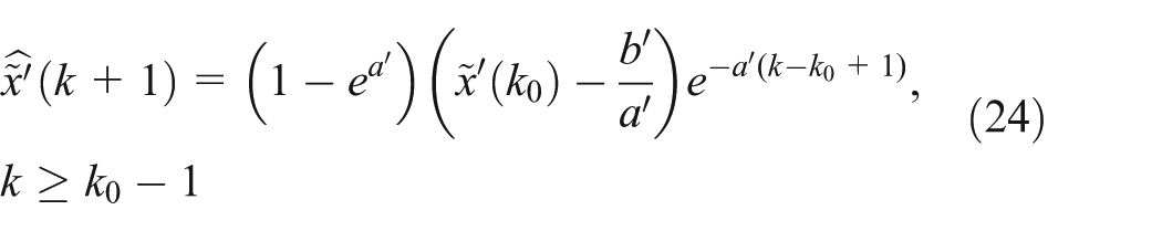
Based on this method of modelling GM(1,1), we can build a GM(1,1) model of the 1-AGO series

Therefore, the GM(1,1) form of the fitted series
Based on the additive modelling idea of seasonal time series, by combining equations (19) and (24), we can obtain the final RC-GMPEM model, which has been corrected using remnants

where
Model applications
Data
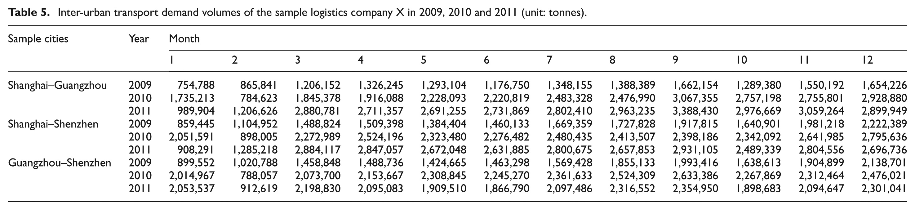
The proposed model is applied to predict the short-term transport demand in between three hub cities for a large five-star transportation logistics company in China, whose major business is domestic road less-than-truckload (LTL) freight transportation between big cities. The data cover all the transport volumes of Shanghai–Guangzhou, Shanghai–Shenzhen and Guangzhou–Shenzhen during a 36-month period (January 2009 to December 2011). The real raw data are shown in Table 5 in Appendix 1. These three time series show a tendency towards irregular periods. Our proposed model is used to analyse the time series.
Modelling results
Let


Based on a confidence level


The main combination models (GMPEMs) are


The prediction accuracy of the three GMPEMs is shown in Table 2.
Prediction accuracy of the three GMPEMs.

GMPEM: GM(1,1)-periodic extension model.
Table 2 shows that the prediction accuracy of the GMPEMs fits the observation series of Shanghai–Guangzhou and Shanghai–Shenzhen well but is weak for Guangzhou–Shenzhen. There is a possibility that the prediction accuracy differences among the different samples could be due to random errors in the time series, and therefore, if feasible, it is necessary to eliminate the random error disturbance adversely affecting the prediction accuracy as much as possible, especially for the time series of Guangzhou–Shenzhen.
We use the method in section ‘Correct the random error of the GMPEM by remnant correction’ to correct the random errors for the three sample time series. The results are as follows:
For Shanghai–Guangzhou, there is the presence of

For Shanghai–Shenzhen, we detect the presence of
For Guangzhou–Shenzhen, there is the presence of

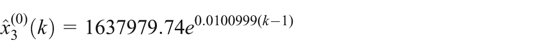
After random error correction for the remnant tail time series of the main combination forecasting model, we can obtain the final combination forecasting models (RC-GMPEMs)

where if
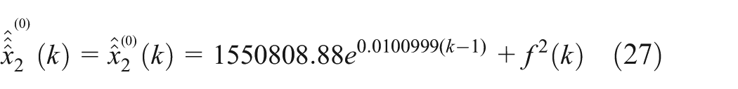

where if
Forecasting results and model comparison
As a comparison analysis of forecasting accuracy in the sample, we use the additive polynomial trend model 16 in equation (29), SARIMA model and RC-GMPEMs to forecast the same time series

where
The forecast results are shown in Figures 2–4. The dominant period of SARIMA models is 13; the predicted values are obtained from forecasting point 14.

Fitted transport demand and actual demand of Shanghai–Guangzhou.
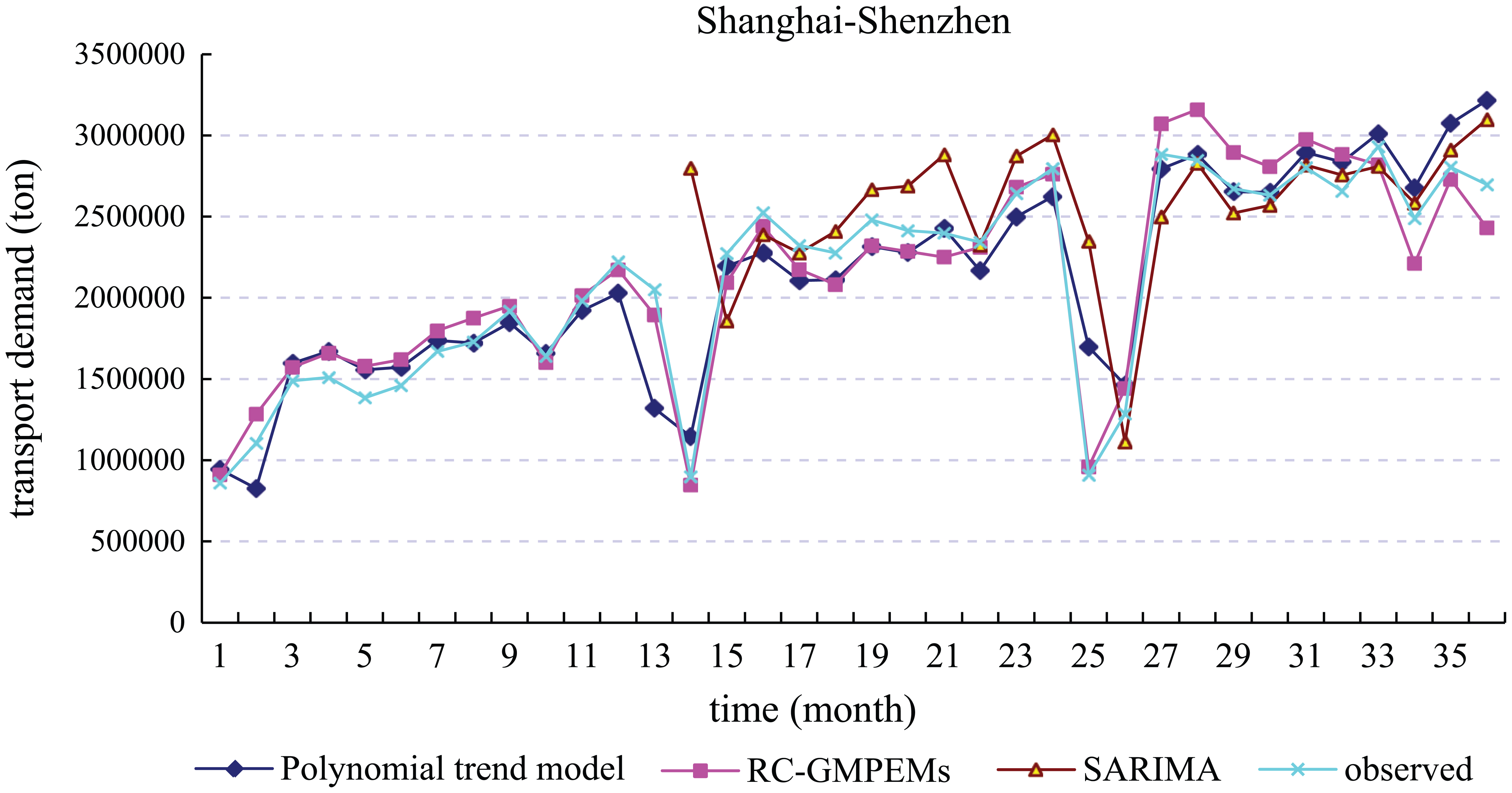
Fitted transport demand and actual demand of Shanghai–Shenzhen.

Fitted transport demand and actual demand of Guangzhou–Shenzhen.
Figures 2–4 show that the RC-GMPEMs have better prediction performance than the other two. Specific criteria, stated by Nelder and Wedderburn,
25
such as the coefficient of determination

where n is the observation number and
Goodness of fit.

RC-GMPEM: GM(1,1)-periodic extension model with remnant correction; SARIMA: Seasonal Autoregressive Integrated Moving Average.
In terms of
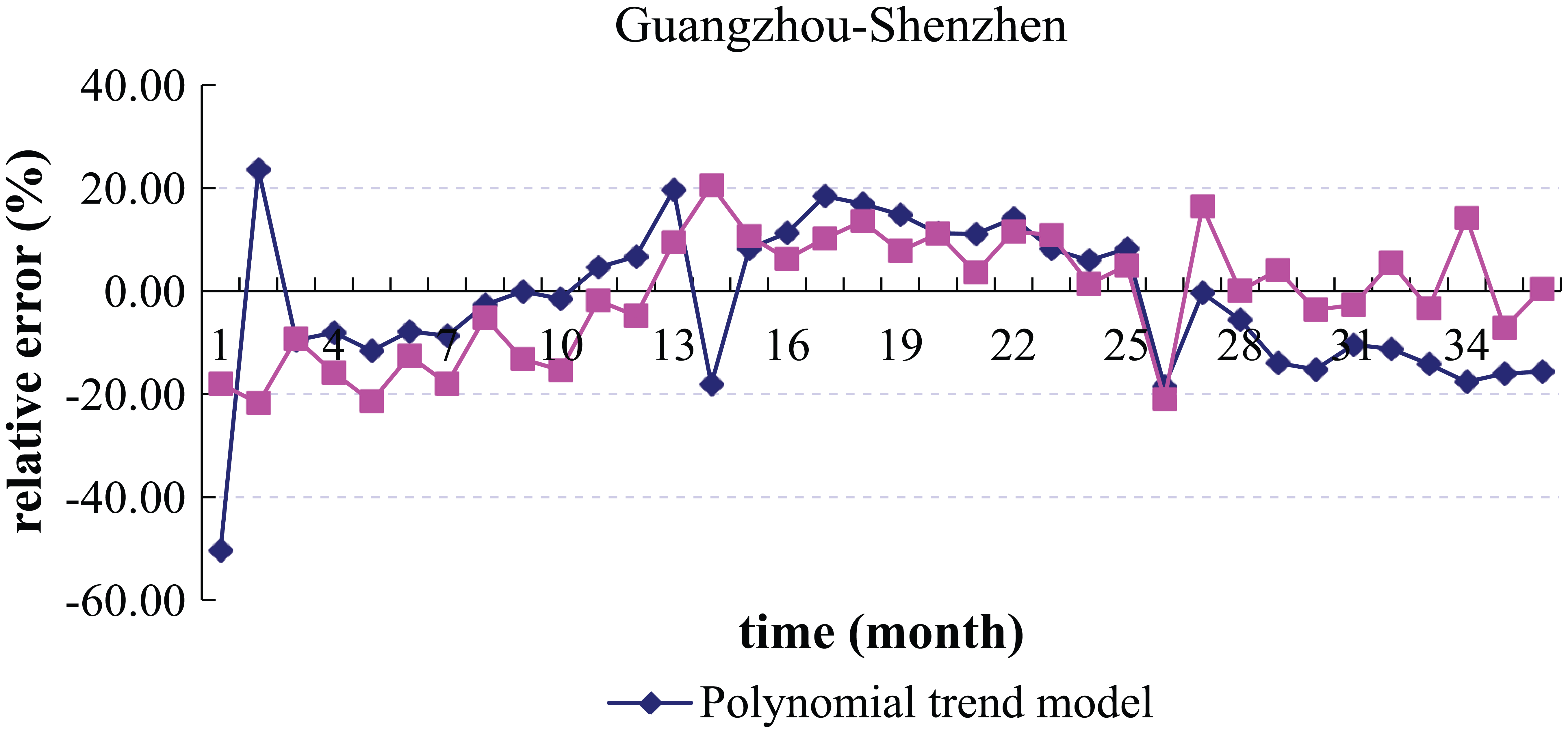
For further comparative analysis, the mean absolute relative error is used as another dimensionless index to measure the forecasting accuracy of the polynomial trend model and the proposed RC-GMPEMs. We computed the relative errors of the polynomial trend models and the RC-GMPEMs. Figures 5–7 show that the relative errors of the RC-GMPEMs are obviously smaller than those of the polynomial trend models.

Relative errors of the forecasted demand of Shanghai–Guangzhou.

Relative errors of the forecasted demand of Shanghai–Shenzhen.
Relative errors of the forecasted demand of Guangzhou–Shenzhen.
The mean absolute relative errors listed in Table 4 show that RC-GMPEMs perform better than the polynomial trend models, which demonstrate that the RC-GMPEMs have advantages over the polynomial trend models in coping with short time series with trend and non-stationary periods by carrying out remnant corrections on the main combination model.
Mean absolute relative errors for the polynomial trend models and RC-GMPEMs.

RC-GMPEM: GM(1,1)-periodic extension model with remnant correction.
Conclusion
Classical transportation economics usually focuses on macro comprehensive transportation demand in a state, a region or in between two cities, which offers a research approach to revealing the relations of transportation demand. These relations are helpful for logistics companies but are insufficient. For an individual logistics company, the market denotes the macroeconomic environment and the transportation industry environment, as well as its own market operation strategies (such as service level, pricing strategy, etc.). Therefore, forecasting the transportation demand of an individual company involved in the market will support the logistics company in making its market operation decision-making. In this article, the grey model GM(1,1) combined with a PEM is used to forecast a company’s short-term transportation demand for two reasons. First, the grey model is used to capture the trend component because the factors affecting a company’s transportation demand are more complicated and fuzzier than those influencing the macro transportation demand. Second, the PEM is chosen to find the implied periods from an observed data series because seasonality is related to the economic cycle but does not coincide with the cycle.
The remnant correction model is used to improve the reliability and validation of the main model. When the same model is applied to different objects (i.e. different observed data series), remnants will be generated, because each market has different influencing factors and changing laws, including trends, period length and fluctuation range. The remnants, which are usually included as the last component of a model, as random perturbation, are often referred to as white noise. The fact is that remnants are related to the reliability and validity of the model. When remnants are large and cannot be ignored, the model should be adjusted until satisfactory reliability and validity are achieved. In this article, prediction accuracy analysis, by checking the remnants of the GM(1,1)-PEM, is performed to determine whether the main model needs adjustment. If the main model needs fixing, GM(1,1) will be used to fit the remnant series, fixing the main model.
The proposed model shows good adaptability in the case study in terms of the choice of the sample company and sample data series. This sample company is a large-scale transportation-oriented logistics company, whose business is an LTL road transportation service in a nationwide hub-and-spoke network in China. The LTL transportation market in China is now clearly divided into two levels. The upper level is a nationwide business, which is taken up by a few large-scale companies similar to the sample one, while numerous Small and Medium-sized Enterprises (SMEs) compete in the remaining market. Competition is fierce, and concentration is very low. As the level of logistics management has increased in recent years, market concentration has slowly grown. The sample company has a good representation of the upper market segmentation. The observed time series cover all the business data of the three origin-destination hub cities of the sample company during a 36-month period (January 2009 to December 2011), during which the national economy had only just recovered from the financial crisis. The forecasting results show that the model has good adaptability to the macroeconomic environment.
Footnotes
Appendix 1
Inter-urban transport demand volumes of the sample logistics company X in 2009, 2010 and 2011 (unit: tonnes).
| Sample cities | Year | Month |
|||||||||||
|---|---|---|---|---|---|---|---|---|---|---|---|---|---|
| 1 | 2 | 3 | 4 | 5 | 6 | 7 | 8 | 9 | 10 | 11 | 12 | ||
| Shanghai–Guangzhou | 2009 | 754,788 | 865,841 | 1,206,152 | 1,326,245 | 1,293,104 | 1,176,750 | 1,348,155 | 1,388,389 | 1,662,154 | 1,289,380 | 1,550,192 | 1,654,226 |
| 2010 | 1,735,213 | 784,623 | 1,845,378 | 1,916,088 | 2,228,093 | 2,220,819 | 2,483,328 | 2,476,990 | 3,067,355 | 2,757,198 | 2,755,801 | 2,928,880 | |
| 2011 | 989,904 | 1,206,626 | 2,880,781 | 2,711,357 | 2,691,255 | 2,731,869 | 2,802,410 | 2,963,235 | 3,388,430 | 2,976,669 | 3,059,264 | 2,899,949 | |
| Shanghai–Shenzhen | 2009 | 859,445 | 1,104,952 | 1,488,824 | 1,509,398 | 1,384,404 | 1,460,133 | 1,669,359 | 1,727,828 | 1,917,815 | 1,640,901 | 1,981,218 | 2,222,389 |
| 2010 | 2,051,591 | 898,005 | 2,272,989 | 2,524,196 | 2,323,480 | 2,276,482 | 2,480,435 | 2,413,507 | 2,398,186 | 2,342,092 | 2,641,985 | 2,795,636 | |
| 2011 | 908,291 | 1,285,218 | 2,884,117 | 2,847,057 | 2,672,048 | 2,631,885 | 2,800,675 | 2,657,853 | 2,931,105 | 2,489,339 | 2,804,556 | 2,696,736 | |
| Guangzhou–Shenzhen | 2009 | 899,552 | 1,020,788 | 1,458,848 | 1,488,736 | 1,424,665 | 1,463,298 | 1,569,428 | 1,855,133 | 1,993,416 | 1,638,613 | 1,904,899 | 2,138,701 |
| 2010 | 2,014,967 | 788,057 | 2,073,700 | 2,153,667 | 2,308,845 | 2,245,270 | 2,361,633 | 2,524,309 | 2,633,386 | 2,267,869 | 2,312,464 | 2,476,021 | |
| 2011 | 2,053,537 | 912,619 | 2,198,830 | 2,095,083 | 1,909,510 | 1,866,790 | 2,097,486 | 2,316,552 | 2,354,950 | 1,898,683 | 2,094,647 | 2,301,041 | |
Acknowledgements
The authors would like to thank the reviewers for their valuable comments and suggestions.
Academic Editor: Hamid Reza Shaker
Declaration of conflicting interests
The author(s) declared no potential conflicts of interest with respect to the research, authorship, and/or publication of this article.
Funding
The author(s) disclosed receipt of the following financial support for the research, authorship, and/or publication of this article: This research was supported by the National Natural Science Foundation of China (NSFC) under grant no. 61203162. This research was also supported in part by the Research and Development Funds of Science and Technology of China Railway Corporation (2013X008).