Sage Journals: Discover world-class research

Abstract

In order to find a proper method to study the flow and sound fields in an axial-flow check valve, the jetting noise at a nozzle is investigated with simulations and experiments. Based on optimization principle, the main channel of the valve body is numerically investigated and optimized twice. The results show that the resistance coefficient and the maximum noise of the valve are decreased by 0.37 and 23.8 dB, respectively, and the head and the tail of the valve plug are optimized when streamline design is employed on the main channel structure of the valve body.

Keywords

Axial-flow check valve flow field sound field optimization experimental

Introduction

Valves are widely used in our life and industry. However, the valve noise brings us lots of energy loss and also disturbs our life. It is necessary to study the noise mechanism in valves and decrease the noise.^1–4 There are many experts and scholars engaged in the related research, achieving good results. PL Jenvey⁵ applied Lighthill’s eighth power of velocity relationship in the special case of noise generated by gas pressure–reducing valves. The experimental results indicated that the acoustic efficiency was decreased for small enclosed jets. TW Lancey⁶ measured noise of air jets with diameters of 0.0794–0.635 cm, with jet exit velocity varying from 54 to 244 m/s. The results are compared to those previously obtained for larger nozzles. Acoustical power spectral density curves were found to be similar to those for the larger nozzles at like velocities. FJ Newton et al.⁷ described a computer system to design trim cages for controlling the flow within gas valves. The results show that the design was simplified and obtained good performance. WJ Rahmeyer⁸ discussed and presented the experimental data for the cavitation noise limit as well as the cavitation limits of incipient, critical, incipient damage, and choking cavitation for the butterfly valves. A noise level of 85 dB was selected as the noise limit. KA El-Shorbagy⁹ investigated valve noise with Lighthill’s acoustic analogy and Curle’s theory for two cases of variable orifice area and variable mass flow rate. The results indicated that monitoring sound levels of valve noise are useful for flow rate measurements and on-line automatic flow control in pipes. A Amini and I Owen¹⁰ changed the design of the original flat plug and seat in gas pressure–reducing valves, finding that a 60° conical plug and seat produced a noise reduction of 12 dB, and the mechanical vibration was eliminated, and the flow capacity was increased by about 25%. J Ryu et al.¹¹ adopted a frequency-domain acoustic analogy to compute internal aerodynamic noise from a quick-opening throttle valve. The prediction of the acoustic pressure level of the quick-opening throttle valve showed good agreement with the existing measurement. The flow-noise generation mechanism was analyzed, finding that the anti-vortex lines play a crucial role in generating the dipolar sound from the unsteady loading of the quick-opening throttle valve. MC Sekhar et al.¹² studied the spin-transfer torque-induced noise in self-biased differential dual spin valves (DDSVs), showing that self-biased DDSV provided a much stronger stability against spin-transfer torque noise than conventional spin valves. D Zhang and colleagues^13,14 confirmed that the asymmetric unstable flow was the root cause of the valve problems such as vibration and failure. C Bolin and A Engeda¹⁵ further studied the mechanisms of valve instability caused by unsteady flows around the valve and the asymmetric unstable flow, noise, and vibration characteristics of the valve.

In the above researches, different theoretical and experimental methods are applied to deeply study the valve noise and feasible suggestions are proposed on its design and manufacturing by experts and scholars. In this work, the noise mechanism of the axial-flow check valve is investigated. A proper numerical method is proposed for computing the noise of axial-flow check valve and the structure is optimized to decrease flow resistance and noise.

Experiments and numerical simulations of aerodynamic noise

Experimental system

As shown in Figure 1, the experimental system consists of a compressor, a gas tank, pressure regulator pipe, a nozzle, and other parts. High-pressure air generated by the compressor will successively flow through the gas tank, the pressure regulator pipe, and the nozzle; finally, it will eject into the ambient space. The mass flow rate is measured by the micromanometer. The inner diameter of the nozzle is 19.05 mm; its structure is shown in Figure 2. The ambient temperature of the laboratory is 16°C. The pressure and temperature of air are 0.5 MPa (gauge pressure) and 24°C in front of the nozzle, respectively, while the local atmospheric pressure is 85 kPa.

Figure 1.

Experimental system.

Figure 2.

Structure of nozzle.

Mathematical model

When the fluid passes through the valve, the noise is mainly produced by the interaction of the fluid and the fluid (or the fluid and the solid). As a result, the basic equations of the flow and the sound field in the valve are expressed as follows:

Navier–Stokes equation

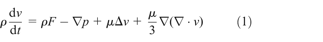
ρ \frac{d v}{d t} = ρ F - \nabla p + μ Δ v + \frac{μ}{3} \nabla (\nabla \cdot v)

(1)

where ρ is the fluid density, v is the fluid velocity, t is the flow time, F is the mass force distribution function, p is the fluid pressure, and µ is the dynamic viscosity.

Lighthill wave equation

\frac{\partial^{2} ρ}{\partial t^{2}} - {a_{0}}^{2} \frac{\partial^{2} ρ}{\partial {x_{i}}^{2}} = \frac{\partial^{2} T_{ij}}{\partial x_{i} x_{j}}

(2)

T_{ij} = ρ u_{i} u_{j} + [(p - p_{0}) - {c_{0}}^{2} (ρ - ρ_{0})] δ_{ij}

(3)

where a₀ is the local sound speed, x_i is the i-axis coordinate, x_j is the j-axis coordinate, T_ij is the Lighthill stress tensor, u_i is the velocity component in i-axis, u_j is the velocity component in j-axis, p₀ is the static pressure, ρ₀ is the density of free flow, and δ_ij is the Kronecker delta.

Ffowcs Williams and Hawkings (FW-H) equation

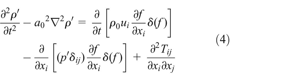
\begin{array}{l} \frac{\partial^{2} ρ^{'}}{\partial t^{2}} - a_{0}^{2} \nabla^{2} ρ^{'} = \frac{\partial}{\partial t} [ρ_{0} u_{i} \frac{\partial f}{\partial x_{i}} δ (f)] \\ - \frac{\partial}{\partial x_{i}} [(p^{'} δ_{i j}) \frac{\partial f}{\partial x_{i}} δ (f)] + \frac{\partial^{2} T_{i j}}{\partial x_{i} \partial x_{j}} \end{array}

(4)

where ρ′ is the perturbation of the fluid density, p′ is the sound pressure, f is the generalized function, and δ(f) is the Dirac function.

The sound pressure level is defined as follows

SPL (dB) = 20 \log | \frac{p}{p_{ref}} |

(5)

where p_ref is the reference sound pressure; p_ref = 20 µPa.

A two-dimensional (2D) axisymmetric model is employed to study the nozzle noise with the software Fluent release 6.3.26.¹⁶ The computational domain is a rectangular region mapped with 3000 × 1000 cells; the grid model is shown in Figure 3. The dimensions of the nozzle are identical with the experimental nozzle. As Reynolds stress (RS) tensor is the root of noise, eddy viscosity method is adopted to solve RS tensor in the standard k – ε (SKE) model, while the higher matrix method is used in the RS model. As a result, the SKE and RS models are chosen as the numerical computational methods because of their different essence. The boundary conditions are as follows: for the inlet, the pressure-inlet boundary is employed, and the gauge total pressure is 50,000 Pa; the turbulent intensity and hydraulic diameter are 10% and 0.0085 m, respectively. For the outlet, the pressure-outlet boundary is adopted, and the gauge pressure is 0 Pa.

Figure 3.

Grid model of the computational domain.

Model verification

Mass flow rates of nozzle

The mass flow rates of the nozzle obtained by the experiments, SKE model, and RS model are shown in Table 1. It is observed that the numerical results have a high agreement with the experiment and the results of the two numerical models are nearly the same.

Table 1.

Flow rates of nozzle obtained by experiments and numerical simulations.

Experiment (kg/s)	SKE model (kg/s)	RS model (kg/s)
0.167	0.166146	0.166691

SKE: standard k – ε; RS: Reynolds stress.

Velocity and temperature distributions along the axis of nozzle

Figure 4 presents the velocity distributions of SKE and RS models along the axis of the nozzle. It is seen from the figure that the velocity distributions of the two models along the axis are quite similar. The differences of the two models are very small in the distance of 0–0.2 m from the nozzle. But when the distance from the nozzle was more than 0.5 m, the velocity of SKE model was slightly higher than RS model. The difference between them is about 2.3%–4.2%.

Figure 4.

Axial velocity distributions of SKE and RS models.

Figure 5 presents the temperature distributions of SKE and RS models along the axis of the nozzle. It is seen from the figure that the temperature of two models along the axis is almost the same. The value and position of the lowest temperature (only 269 K) in the temperature field are nearly the same. Despite some differences between the two models at the distance of 0.2–0.3 m from the nozzle, the difference between them is about 1.1%–1.7%.

Figure 5.

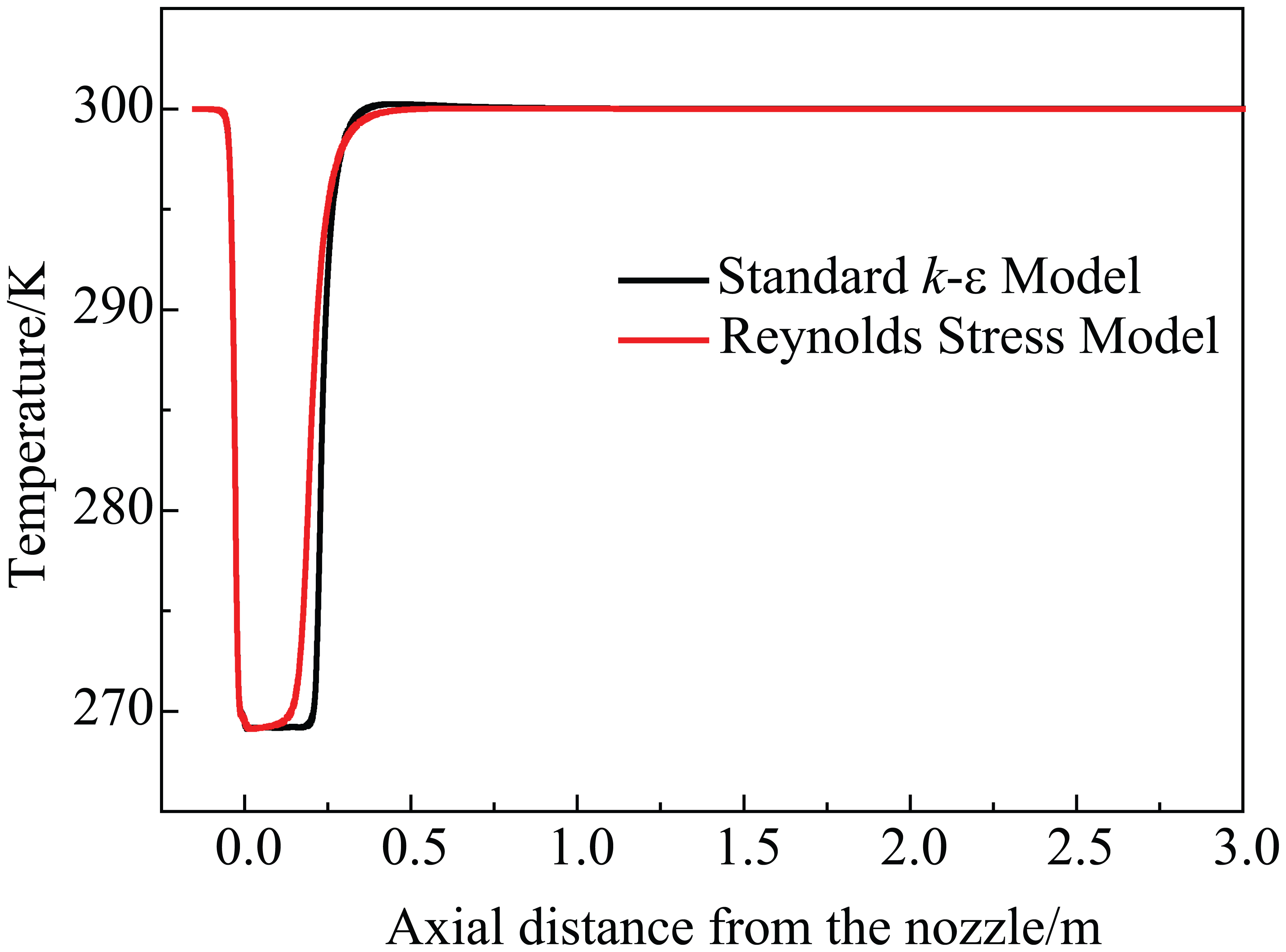
Axial temperature distributions of SKE and RS models.

Sound fields

Figure 6 presents the measured results of jet noise power levels after eliminating background noise. Figure 7 presents sound power levels of SKE and RS models. Compare results in Figures 6 and 7; the measured sound field is higher than 90 dB, while the numerical result of the broadband noise source at the corresponding location is only about 20 dB. Since the difference is huge, the numerical results do not have practical guiding value. The data of the corresponding points in the injection region are analyzed; the radius and length of the injection region are 1 and 5 m, respectively. It is seen that the measured data and the numerical results have the same trend, but the numerical results are lower about 8 dB than the measured results.

Figure 6.

Measured results of jet noise power levels.

Figure 7.

Sound power levels of SKE and RS models along the axis of nozzle.

Figures 8 and 9 present the sound power–level distributions of SKE and RS models, respectively. It is seen that the sound fields of the two numerical models are roughly similar. This is due to the similar governing equations in the two models. It can also be seen that the maximum sound power level of SKE model is 148 dB, while the maximum sound power level of RS model is 144 dB. The main reason of the differences is that the RS term is solved by different methods. As a result, there are differences in the turbulent kinetic energy in the high turbulent region, as shown in Figure 10.

Figure 8.

Contours of sound power levels in SKE model.

Figure 9.

Contours of sound power levels in RS model.

Figure 10.

Turbulent kinetic energy of SKE and RS models.

Optimization of axial-flow check valve

When noise in a limited space like valves is simulated, these regions are directly affected by the turbulent zone. Despite the experimental and numerical results being different, they have the same trend. When the quantitative prediction of noise is not required, a numerical method could be adopted to qualitatively analyze the noise field.

In this work, the optimized object is an axial-flow check valve, using the streamlined valve plug as the opening and closing components of the valve; its structure is shown in Figure 11. The optimization goal is to reduce flow resistance and noise.

Figure 11.

The structure of axial-flow check valve.

Optimization principles of flow field in axial-flow check valve

When the fluid flows through the valve, the resistance of the fluid mainly comes from two aspects as follows: (1) one part is friction resistance between the fluid and the solid boundary caused by the viscous effects. (2) As the solid surface is non-flat solid surface, the boundary layer is out of the wall, and the fluid detached from the wall forms a low-pressure vortex, resulting in an additional resistance, namely, pressure drag. As a result, the measures for decreasing valve resistance are expressed as follows: (1) in order to make the flow to be laminar, the front part of valve surface should be kept as smooth as possible. (2) For matching with the structure of valve plug, the structure of the outer channel is optimized so that the border is located in a favorable pressure gradient region, eliminating the possibility of boundary layer separation. (3) In the transition region from laminar flow to turbulent flow, the disturbance is intensified for making boundary layer transform into turbulent flow in advance, decreasing the boundary layer separation and the pressure drag.

Accuracy test of numerical simulation

As the boundary layer separation point is related to solid shapes, wall pressure gradient, and other factors, it is difficult to determine the specific separation location and pressure drop by theoretical formula, so the numerical method is employed to compute separation point and flow resistance. Considering the accuracy of the numerical method is also affected by various factors, it needs to be verified.

To determine whether the numerical method can accurately calculate the boundary layer separation point, the flow around the cylinder is simulated. The calculation parameters are as follows: the viscosity and density of air are 1.7894 × 10⁻⁵ Pa s and 1.225 kg/m³, respectively, and the diameter of the cylinder is 0.007 m. A re-normalization group (RNG) model is adopted. The grid near the wall is refined and the enhanced wall model is adopted. The Reynolds number of the inlet in the calculation region is 3 × 10⁶, and the characteristic diameter is the diameter of the cylinder.

It can be concluded from Figures 12 –16 that the numerical pressure distribution is highly consistent with the experimental data.^17–19Figures 14 and 15 show that the boundary layer separates at 140° under turbulence, and it is verified by the experimental and simulation results of other researchers.^17–19 The drag coefficient around the cylinder is 12, having a good agreement with the experimental data.^20–22

Figure 12.

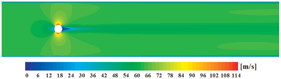
Flow velocity distribution around the cylinder.

Figure 13.

Pressure distribution around the cylinder.

Figure 14.

Streamline around the surface of a cylinder.

Figure 15.

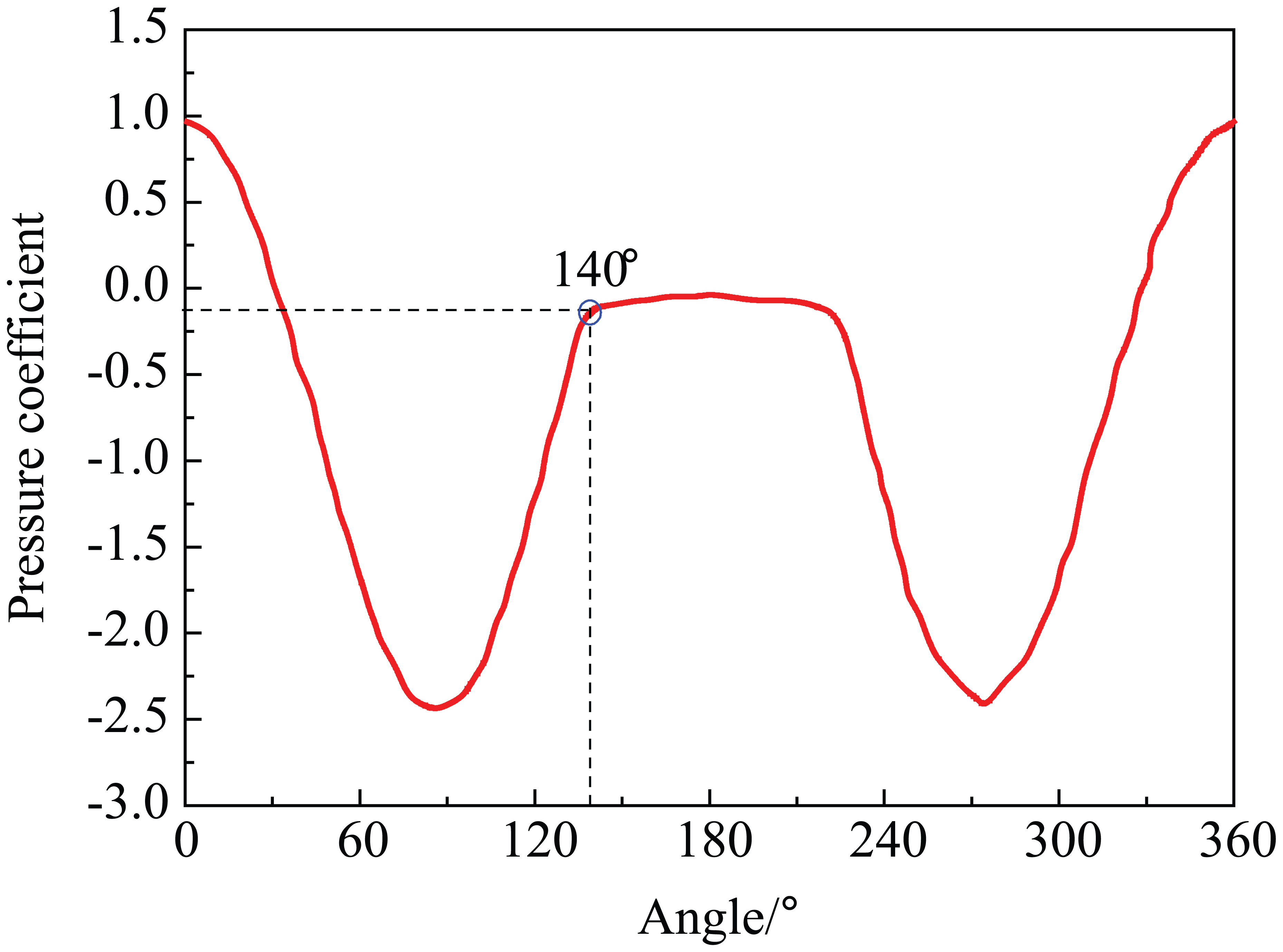
Pressure coefficient of the cylinder surface.

Figure 16.

Drag coefficient of the cylinder surface.

Optimization results

Three structures of valve

Figure 17 presents two structures of the valve. In the figure, the structure unrelated to or having little impact on flow, such as springs, fixed tendons, and other details, is ignored, while the main channel mostly affects the flow resistance. The black line represents the traditional check valve (valve A). The red line stands for the streamlined valve (valve B). Compare with valve A, the line of valve plug is designed into streamline and the line of inner wall in the valve body is expanded for maintaining the cross-sectional area of flow constant. However, the numerical results of valve B show that boundary layer separation and vortex flow still exist at the rear of valve plug and the entrance of valve plug and the channel. As a result, the head and tail of valve plug are optimized, and the resulting structure (valve C) is shown in Figure 18.

Figure 17.

Two different structures of the valve.

Figure 18.

3D structure of valve C: (a) the inner wall of valve body and (b) the valve plug.

Pressure fields in three valves

Figure 19 presents the pressure fields in the three valve channels. It can be seen from the figure that the three pressure fields are similar and the pressure gradually decreases from the inlet to the outlet, and the maximum pressure locates at the center of the positive side of valve plug. The maximum pressure of valve A is 392 Pa, while that of valve B and valve C are 350 and 322 Pa, respectively. In all, the passage formed by valve plug and sealing surface of valve seat plays an important role in the pressure drop.

Figure 19.

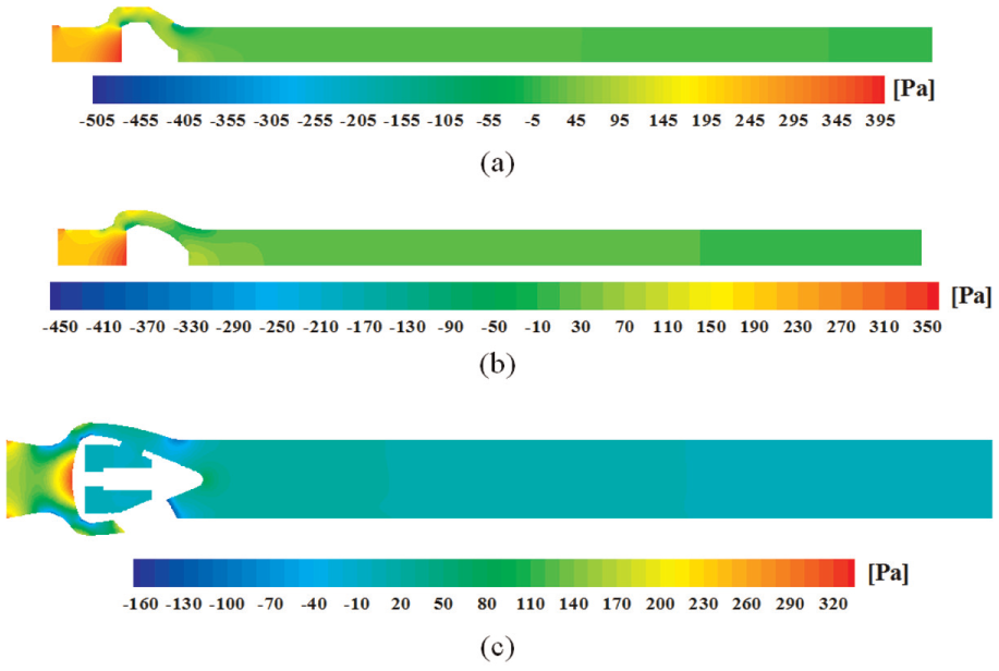
Contours of pressure fields in three valve channels: (a) valve A, (b) valve B, and (c) valve C.

Flow field in three valves

Figure 20 presents the flow field in three valve channels. As shown in Figure 20, the plug of valve A has a concave curve, leading to the expansion of channel section. As a result, the boundary layer of the valve plug surface goes away from the wall, forming vortexes. The equal cross-sectional design was used in valve B, keeping the pressure gradient near the wall in the inverse pressure region and wall boundary layer attached to the surface of valve plug. The channel section of entrance in valve B expands too fast, forming a swirl flow at the entrance and unfavorable for decreasing flow resistance. Valve C has no shortcomings as above.

Figure 20.

Flow fields in three valve channels: (a) valve A, (b) valve B, and (c) valve C.

The flow resistance in three valves

Figure 21 presents the flow resistance coefficient of three valves. It can be seen from the histogram that the flow resistance coefficient decreases from 1.84 to 1.37 with two optimizations. This is because the streamline design is employed to decrease the resistance force of the valve.

Figure 21.

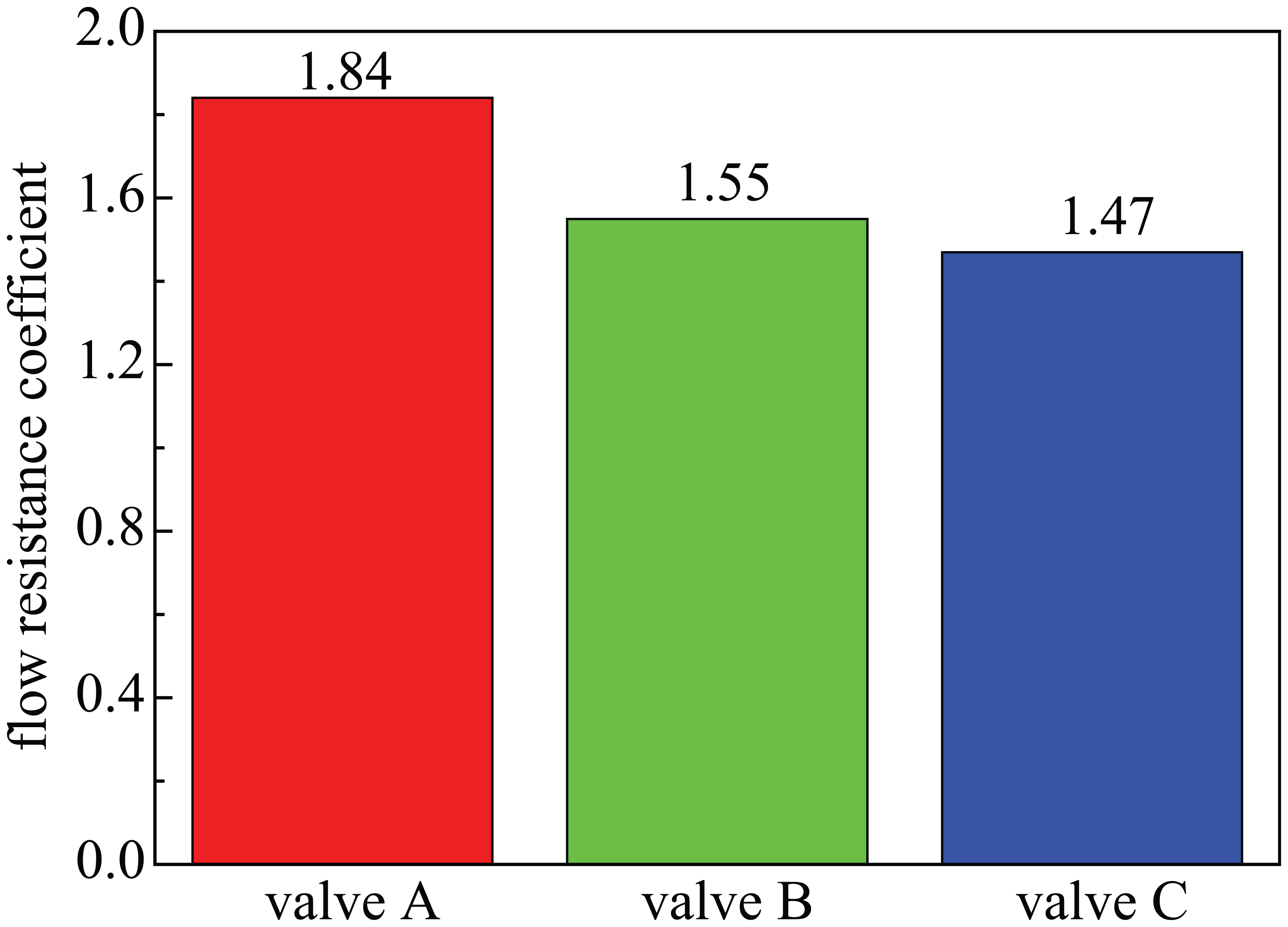
Flow resistance coefficient of three valves.

Noise power levels in three valves

Figure 22 presents the noise power levels in three valves. It is found that the maximum noise level decreases with the optimized valve plug, and the maximum noise levels of valve A, valve B, and valve C are 95.4, 93.8, and 71.6 dB, respectively. The decrease in noise power levels stands for the decrease in energy loss of fluid. It should be contributed to the streamline design for decreasing the resistance force.

Figure 22.

Noise power level in three valves: (a) valve A, (b) valve B, and (c) valve C.

Conclusion

In this work, the jetting noise at a nozzle is investigated with simulations and experiments The results show that the numerical method can be adopted to qualitatively analyze the noise field because of the same trend between the experimental and numerical results. As a result, the software Fluent is adopted to study the flow and sound fields of an axial-flow check valve. Based on optimization principle, the main channel structure of the valve body is optimized twice; it is shown that the resistance coefficient and maximum noise of valve decrease by 0.37 and 23.8 dB, respectively, when streamline design is employed in the main channel structure of valve body and the head and tail of the valve plug are optimized.

Footnotes

Academic Editor: Takahiro Tsukahara

Declaration of conflicting interests

The author(s) declared no potential conflicts of interest with respect to the research, authorship, and/or publication of this article.

Funding

The author(s) received no financial support for the research, authorship, and/or publication of this article.

References

Beranek

Vér

IL.

Noise and vibration control engineering. New York: John Wiley & Sons, 1992.

KW.

Control valve noise. ISA T 1994; 33: 275–286.

Kim

Lee

DJ.

Numerical analysis of internal combustion engine intake noise with a moving piston and a valve. J Sound Vib 2001; 241: 895–912.

Nesbitt

Handbook of valves and actuators: valves manual international. Oxford: Butterworth-Heinemann, 2011.

Jenvey

PL.

Gas pressure reducing valve noise. J Sound Vib 1975; 41: 506–509.

Lancey

TW.

Noise from small air jets and a quiet valve. J Sound Vib 1978; 57: 35–40.

Newton

Mountford Laxon

WR.

Design of low-noise gas valves. Comput Aided Design 1977; 9: 135–140.

Rahmeyer

WJ.

Cavitation noise from butterfly valves. Nucl Eng Des 1982; 72: 297–301.

El-Shorbagy

KA.

An investigation into noise radiation from flow control valves with particular reference to flow rate measurement. Appl Acoust 1983; 16: 169–181.

10.

Amini

Owen

A practical solution to the problem of noise and vibration in a pressure-reducing valve. Exp Therm Fluid Sci 1995; 10: 136–141.

11.

Ryu

Cheong

Kim

. Computation of internal aerodynamic noise from a quick-opening throttle valve using frequency-domain acoustic analogy. Appl Acoust 2005; 66: 1278–1308.

12.

Sekhar

Tran

Wang

. Enhanced stability against spin torque noise in current perpendicular to the plane self-biased differential dual spin valves. J Magn Magn Mater 2015; 374: 740–743.

13.

Zhang

Engeda

Venturi valves for steam turbines and improved design considerations. Proc IMechE, Part A: J Power and Energy 2003; 217: 219–230.

14.

Zhang

Engeda

Hardin

. Experimental study of steam turbine control valves. Proc IMechE, Part C: J Mechanical Engineering Science 2004; 218: 493–507.

15.

Bolin

Engeda

Analysis of flow-induced instability in a redesigned steam control valve. Appl Therm Eng 2015; 83: 40–47.

16.

Fluent Inc. Fluent release 6.3.26 user guide. Fluent Inc., 2006, Canonsburg.

17.

Hoffman

. Simulating drag crisis for a sphere using skin friction boundary conditions. In: Proceedings of the European conference on computational fluid dynamics—ECCOMAS CFD 2006, Egmond aan Zee, The Netherlands, 5–8 September 2006. The Netherlands: Delft University of Technology; European Community on Computational Methods in Applied Sciences.

18.

Singh

Mittal

Flow past a cylinder: shear layer instability and drag crisis. Int J Numer Meth Fl 2005; 47: 75–98.

19.

Williamson

CHK

. Vortex dynamics in the cylinder wake. Annu Rev Fluid Mech 1996; 28: 477–539.

20.

Bloor

MS.

The transition to turbulence in the wake of a circular cylinder. J Fluid Mech 1964; 19: 290–304.

21.

Gerrard

JH.

The wakes of cylindrical bluff bodies at low Reynolds number. Philos T R Soc S: A 1978; 288: 351–382.

22.

Wei

Smith

CR.

Secondary vortices in the wake of circular cylinders. J Fluid Mech 1986; 169: 513–533.

Numerical and experimental research of flow and sound fields in an axial-flow check valve and its optimization

Abstract

Keywords

Introduction

Experiments and numerical simulations of aerodynamic noise

Experimental system

Mathematical model

Model verification

Mass flow rates of nozzle

Velocity and temperature distributions along the axis of nozzle

Sound fields

Optimization of axial-flow check valve

Optimization principles of flow field in axial-flow check valve

Accuracy test of numerical simulation

Optimization results

Three structures of valve

Pressure fields in three valves

Flow field in three valves

The flow resistance in three valves

Noise power levels in three valves

Conclusion

Footnotes

Declaration of conflicting interests

Funding

References