Rigid–elastic-thermal coupling dynamics and its application

Abstract

Spacecraft dynamics belongs to rigid–elastic coupling dynamics in general. If thermal stress and thermal effect are further considered, it will cause the more complex rigid–elastic-thermal coupling dynamics. For the aforementioned kind of coupling dynamics, it is difficult to establish the basic equations directly. It has proved that a suitable way to study complex coupling problems is by work–energy theorem and the law of conversation of energy. Using the energy method, Hamilton principle of rigid–elastic-thermal coupling dynamics is established. The stationary value conditions of Hamilton principle of rigid–elastic-thermal coupling dynamics are derived. The physical meaning of the stationary value conditions is indicated. As an application of rigid–elastic-thermal coupling dynamics, the actual example of spacecraft is given to reveal that there existed thermal stiffening or softening problems in rigid–elastic-thermal coupling dynamics, just like dynamic hardening or softening problems in spacecraft dynamics.

Introduction

With the continuous improvement of the speed of aircrafts, the thermal barrier problem has appeared in flight dynamics; thermal stress and thermal effect problems have also been paid more and more attention in academia. As an example of spacecraft in flight, aircraft will be subjected to the most extreme conditions, which temperature can be from more than 200 degrees below zero Celsius to thousands of degrees. Although the development of thermal control technology has greatly reduced the influence of thermal environment on the aircraft structure strength, it is still a problem that should be considered.^1,2 Similarly, with the continuous development of nuclear technology and engineering, a series of theory and practical problems related to thermal stress and thermal effect have been put forward. Due to the importance of the problem, it is still a hot research field until now.^3–7

Generally, spacecraft dynamics belongs to rigid–elastic coupling dynamics. If thermal stress and thermal effect are considered further, it may cause more complicated rigid–elastic-thermal coupling dynamics. Ma et al. ⁸ point out that because of the complexity of flexible multi-body configuration, recent study to solve the problems of flexible multi-body dynamics mainly depends on the numerical and quantitative methods almost no one involves in the analytical discussion. It is unfavorable to understand profoundly the essence of nonlinear mechanics of the system and to predict the feature of overall dynamics of system. Therefore, it needs to study theoretical analysis of flexible multi-body system. This is a very complex problem and it takes a very long time to solve this problem. Inspired by the above discussion, the analytic solutions of rigid–elastic-thermal coupling dynamics are carried out in this article. For this kind of coupling dynamics, it is so hard to establish the governing equation. It is proved that it is a suitable way to study the coupling problems by work–energy theorem and the law of conversation of energy.^9–11

Hamilton principle of rigid–elastic-thermal coupling dynamics is established by the energy method. The stationary value conditions of Hamilton principle of rigid–elastic-thermal coupling dynamics are derived. The physical meaning of the stationary value conditions is indicated. As an application of rigid–elastic-thermal coupling dynamics, the actual example of spacecraft is given to reveal that there existed thermal stiffening or softening problems in rigid–elastic-thermal coupling dynamics, just like dynamic hardening or softening problems in spacecraft dynamics.^12–15

Hamilton principle of rigid–elastic-thermal dynamics

Because of complexity within this problem, this article adopts tensor as follows.^16,17

In rigid–elastic-thermal system, the sum radius-vector of a point can be expressed as $\mathit{R}={\mathit{X}}^c+\mathit{x}+\mathit{u}$ , where ${\mathit{X}}^c$ is the radius-vector of the mass center, $\mathit{x}$ is the radius-vector from the center to any point when rigid–elastic-thermal system is regarded as the rigid body, and $\mathit{u}$ is the elastic displacement of the point, as shown in Figure 1. Then, $\mathit{X}={\mathit{X}}^c+\mathit{x}$ . Here, $\mathbf{\theta }$ is the angle when rigid–elastic-thermal system is regarded as the rigid body or is a pseudo-coordinate. Therefore, rigid–elastic-thermal system has velocity of rigid body $(d\mathit{X}/\mathrm{dt})=(d{\mathit{X}}^c/\mathrm{dt})+(d\mathit{x}/\mathrm{dt})$ and also has deformable velocity $(d\mathit{u}/\mathrm{dt})=(\partial \mathit{u}/\partial t)+(d\mathbf{\theta }/\mathbf{dt})\mathbf{\times }\mathit{u}$ (where × is the vector of multiplication cross symbol). The cross-link between the velocity of deformable body and rotational rigid body should be noted here. The vector $\mathit{x}$ is the distance from the mass center to any point for the rigid body in our mechanical model. Furthermore, the distances of any two points in the rigid body are constants, that is, $(\partial \mathit{x}/\partial t)=0$ . Applying the Coriolis rotational theorem, we have $(d\mathit{x}/\mathrm{dt})=(\partial \mathit{x}/\partial t)+(d\mathbf{\theta }/\mathbf{dt})\mathbf{\times }\mathit{x}\mathbf{=}(\mathbf{d}\mathbf{\theta }/\mathbf{dt})\mathbf{\times }\mathit{x}$ ; therefore

$$\begin{array}{c}\multicolumn{1}{c}{\frac{d\mathit{R}}{\mathrm{dt}}=\frac{d{\mathit{X}}^c}{\mathrm{dt}}+\frac{d\mathit{x}}{\mathrm{dt}}+\frac{d\mathit{u}}{\mathrm{dt}}}\\ \multicolumn{1}{c}{\frac{d\mathit{x}}{\mathrm{dt}}=\frac{\partial \mathit{x}}{\partial t}+\frac{d\mathbf{\theta }}{\mathrm{dt}}\times \mathit{x}=\frac{d\mathbf{\theta }}{\mathrm{dt}}\times \mathit{x}}\\ \multicolumn{1}{c}{\frac{d\mathit{u}}{\mathrm{dt}}=\frac{\partial \mathit{u}}{\partial t}+\frac{d\mathbf{\theta }}{\mathrm{dt}}\times \mathit{u}}\\ \multicolumn{1}{c}{\frac{d\mathit{R}}{\mathrm{dt}}=\frac{d{\mathit{X}}^c}{\mathrm{dt}}+\frac{d\mathbf{\theta }}{\mathrm{dt}}\times \mathit{x}+\frac{\partial \mathit{u}}{\partial t}+\frac{d\mathbf{\theta }}{\mathrm{dt}}\times \mathit{u}}\end{array}$$

(1)

Figure 1.

Mechanical model.

Because of

$$\begin{array}{c}\multicolumn{1}{c}{\frac{d\mathit{R}}{\mathrm{dt}}·\frac{d\mathit{R}}{\mathrm{dt}}=(\frac{d\mathit{X}}{\mathrm{dt}}+\frac{d\mathit{u}}{\mathrm{dt}})·(\frac{d\mathit{X}}{\mathrm{dt}}+\frac{d\mathit{u}}{\mathrm{dt}})}\\ \multicolumn{1}{c}{=\frac{d\mathit{X}}{\mathrm{dt}}·\frac{d\mathit{X}}{\mathrm{dt}}+2\frac{d\mathit{X}}{\mathrm{dt}}·\frac{d\mathit{u}}{\mathrm{dt}}+\frac{d\mathit{u}}{\mathrm{dt}}·\frac{d\mathit{u}}{\mathrm{dt}}}\end{array}$$

(2)

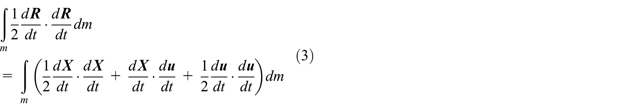
The kinetic energy is

$$\begin{array}{c}\multicolumn{1}{c}{\underset{m}{\int }\frac{1}{2}\frac{d\mathit{R}}{\mathrm{dt}}·\frac{d\mathit{R}}{\mathrm{dt}}\mathrm{dm}}\\ \multicolumn{1}{c}{=\underset{m}{\int }(\frac{1}{2}\frac{d\mathit{X}}{\mathrm{dt}}·\frac{d\mathit{X}}{\mathrm{dt}}+\frac{d\mathit{X}}{\mathrm{dt}}·\frac{d\mathit{u}}{\mathrm{dt}}+\frac{1}{2}\frac{d\mathit{u}}{\mathrm{dt}}·\frac{d\mathit{u}}{\mathrm{dt}})\mathrm{dm}}\end{array}$$

(3)

or

$$\begin{array}{c}\multicolumn{1}{c}{\underset{V}{\int \int \int }\frac{1}{2}\rho \frac{d\mathit{R}}{\mathrm{dt}}·\frac{d\mathit{R}}{\mathrm{dt}}\mathrm{dV}}\\ \multicolumn{1}{c}{=\underset{V}{\int \int \int }(\frac{1}{2}\rho \frac{d\mathit{X}}{\mathrm{dt}}·\frac{d\mathit{X}}{\mathrm{dt}}+\rho \frac{d\mathit{X}}{\mathrm{dt}}·\frac{d\mathit{u}}{\mathrm{dt}}+\frac{1}{2}\rho \frac{d\mathit{u}}{\mathrm{dt}}·\frac{d\mathit{u}}{\mathrm{dt}})\mathrm{dV}}\end{array}$$

(4)

For rigid–elastic-thermal system, if we think that the external forces on the deformable body (including body force f and surface force T ) are the conservative forces, which also lead to the conservative force on the rigid body, that is, the principal force F and the principal couple M acting on the mass center are the conservative generalized forces. Based on work–energy theorem and the law of conversation of energy, Hamilton principle of rigid–elastic-thermal coupled dynamics can be expressed as

$$\begin{array}{c}\multicolumn{1}{c}{{\pi }_{H1}=\underset{t_0}{\overset{t_1}{\int }}[\underset{m}{\int }(\frac{1}{2}\frac{d\mathit{X}}{\mathrm{dt}}·\frac{d\mathit{X}}{\mathrm{dt}}+\frac{d\mathit{X}}{\mathrm{dt}}·\frac{d\mathit{u}}{\mathrm{dt}}+\frac{1}{2}\frac{d\mathit{u}}{\mathrm{dt}}·\frac{d\mathit{u}}{\mathrm{dt}})\mathrm{dm}-{\pi }_1^{*}+\mathit{F}·{\mathit{X}}^c+\mathit{M}·\mathbf{\theta }]\mathrm{dt}}\\ \multicolumn{1}{c}{=\underset{t_0}{\overset{t_1}{\int }}[\underset{V}{\int \int \int }(\frac{1}{2}\rho \frac{d\mathit{X}}{\mathrm{dt}}·\frac{d\mathit{X}}{\mathrm{dt}}+\rho \frac{d\mathit{X}}{\mathrm{dt}}·\frac{d\mathit{u}}{\mathrm{dt}}+\frac{1}{2}\rho \frac{d\mathit{u}}{\mathrm{dt}}·\frac{d\mathit{u}}{\mathrm{dt}})\mathrm{dV}-{\pi }_1^{*}+\mathit{F}·{\mathit{X}}^c+\mathit{M}·\mathbf{\theta }]\mathrm{dt}}\end{array}$$

(5)

$$\begin{array}{c}\multicolumn{1}{c}{{\pi }_1^{•}=\underset{t_0}{\overset{t_1}{\int }}\{\underset{V}{\int \int \int }[(\frac{1}{2}\nabla \mathit{u}+\frac{1}{2}\mathit{u}\nabla +\frac{1}{2}\nabla \mathit{u}·\mathit{u}\nabla )A-\frac{\partial A(\frac{1}{2}\nabla \mathit{u}+\frac{1}{2}\mathit{u}\nabla +\frac{1}{2}\nabla \mathit{u}·\mathit{u}\nabla )}{\partial (\frac{1}{2}\nabla \mathit{u}+\frac{1}{2}\mathit{u}\nabla +\frac{1}{2}\nabla \mathit{u}·\mathit{u}\nabla )}:\mathbf{\delta }\mathbf{\alpha }\mathbf{\Delta }\mathbf{T}-\mathit{f}\mathbf{·}\mathit{u}]\mathrm{dV}-\int \underset{S_{\sigma }}{\int }\mathit{T}·\mathit{u}\mathrm{dS}\}\mathrm{dt}}\end{array}$$

(6)

Prerequisite is

$$\mathit{u}-\overline{\mathit{u}}=0$$

(7)

According to Lu ¹⁸

$$\begin{array}{c}\multicolumn{1}{c}{\underset{m}{\int }\frac{1}{2}\frac{d\mathit{X}}{\mathrm{dt}}·\frac{d\mathit{X}}{\mathrm{dt}}\mathrm{dm}=\underset{m}{\int }\frac{1}{2}\frac{d{\mathit{X}}^c}{\mathrm{dt}}·\frac{d{\mathit{X}}^c}{\mathrm{dt}}\mathrm{dm}}\\ \multicolumn{1}{c}{+\underset{m}{\int }\frac{d{\mathit{X}}^c}{\mathrm{dt}}·(\frac{d\mathbf{\theta }}{\mathrm{dt}}\times \mathit{x})\mathrm{dm}+\underset{m}{\int }\frac{1}{2}{(\frac{d\mathbf{\theta }}{\mathrm{dt}}\times \mathit{x})}^2\mathrm{dm}}\\ \multicolumn{1}{c}{=\underset{m}{\int }\frac{1}{2}\frac{d{\mathit{X}}^c}{\mathrm{dt}}·\frac{d{\mathit{X}}^c}{\mathrm{dt}}\mathrm{dm}+\frac{1}{2}\frac{d\mathbf{\theta }}{\mathrm{dt}}·{\mathit{H}}^c}\end{array}$$

(8)

Thus, Hamilton principle of rigid–elastic-thermal system dynamics can be rewritten as

$$\begin{array}{c}\multicolumn{1}{c}{{\pi }_{H1}=\underset{t_0}{\overset{t_1}{\int }}[\underset{m}{\int }(\frac{1}{2}\frac{d{\mathit{X}}^c}{\mathrm{dt}}·\frac{d{\mathit{X}}^c}{\mathrm{dt}}+\frac{d\mathit{X}}{\mathrm{dt}}·\frac{d\mathit{u}}{\mathrm{dt}}+\frac{1}{2}\frac{d\mathit{u}}{\mathrm{dt}}·\frac{d\mathit{u}}{\mathrm{dt}})\mathrm{dm}+\frac{1}{2}\frac{d\mathbf{\theta }}{\mathrm{dt}}·{\mathit{H}}^c-{\pi }_1+\mathit{F}·{\mathit{X}}^c+\mathit{M}·\mathbf{\theta }]\mathrm{dt}}\\ \multicolumn{1}{c}{=\underset{t_0}{\overset{t_1}{\int }}[\underset{V}{\int \int \int }(\frac{1}{2}\rho \frac{d{\mathit{X}}^c}{\mathrm{dt}}·\frac{d{\mathit{X}}^c}{\mathrm{dt}}+\rho \frac{d\mathit{X}}{\mathrm{dt}}·\frac{d\mathit{u}}{\mathrm{dt}}+\frac{1}{2}\rho \frac{d\mathit{u}}{\mathrm{dt}}·\frac{d\mathit{u}}{\mathrm{dt}})\mathrm{dV}+\frac{1}{2}\frac{d\mathbf{\theta }}{\mathrm{dt}}·{\mathit{H}}^c-{\pi }_1^{*}+\mathit{F}·{\mathit{X}}^c+\mathit{M}·\mathbf{\theta }]\mathrm{dt}}\end{array}$$

(9)

$$\begin{array}{c}\multicolumn{1}{c}{{\pi }_1^{•}=\underset{t_0}{\overset{t_1}{\int }}\{\underset{V}{\int \int \int }[A(\frac{1}{2}\nabla \mathit{u}+\frac{1}{2}\mathit{u}\nabla +\frac{1}{2}\nabla \mathit{u}·\mathit{u}\nabla )-\frac{\partial A(\frac{1}{2}\nabla \mathit{u}+\frac{1}{2}\mathit{u}\nabla +\frac{1}{2}\nabla \mathit{u}·\mathit{u}\nabla )}{\partial (\frac{1}{2}\nabla \mathit{u}+\frac{1}{2}\mathit{u}\nabla +\frac{1}{2}\nabla \mathit{u}·\mathit{u}\nabla )}:\mathbf{\delta }\mathbf{\alpha }\mathbf{\Delta }\mathbf{T}-\mathit{f}\mathbf{·}\mathit{u}\mathbf{]}\mathbf{dV}-\mathbf{\int }\underset{{\mathbf{S}}_{\mathbf{\sigma }}}{\int }\mathit{T}\mathbf{·}\mathit{u}\mathbf{dS}\mathbf{\}}\mathbf{dt}}\end{array}$$

(10)

Prerequisite is

$$\mathit{u}-\overline{\mathit{u}}=0(\mathrm{on}{s}_u)$$

(11)

where u and $\overline{\mathit{u}}$ are the displacement vector and boundary displacement vector, respectively; V is the volume; $s_{\sigma }$ and s_u are the boundary stress and boundary displacement, respectively; A is the strain energy function; t, m, and ρ are the time, mass, and mass density, respectively; ∇ is the Hamiltonian operator. ${\mathit{H}}^c=\mathit{J}·(d\mathbf{\theta }/\mathbf{dt})$ is the moment of momentum with respect to mass center; ${\mathit{H}}^c=\mathit{J}·(d\mathbf{\theta }/\mathbf{dt})$ , notes ${\mathit{H}}^c(\mathbf{\theta })$ . J is the moment of inertia to mass center. Note that $\mathbf{\delta }$ is the Kronecker symbol and $\delta$ is the variational symbol. $\alpha$ and $\Delta T$ are the linear expansion coefficients of the material and variation in temperature field, respectively.

Stationary value conditions of Hamilton principle of rigid–elastic-thermal coupling dynamics

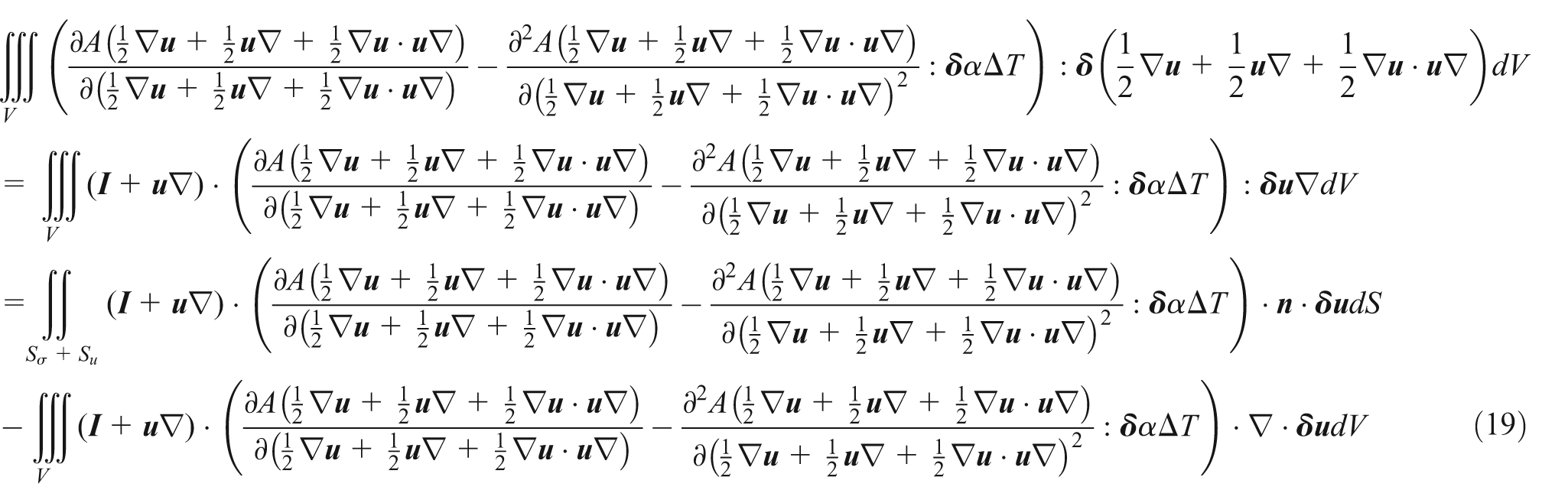
Hu ¹⁹ pointed out that the best way for verifying variational principle is to derive its stationary value conditions. So the following work is focused on obtaining the stationary value conditions of Hamilton principle of rigid–elastic-thermal coupling dynamics.

Let $\delta {\pi }_{H1}=0$ , we obtain

$$\begin{array}{c}\multicolumn{1}{c}{\delta {\pi }_{H1}=\delta \underset{t_0}{\overset{t_1}{\int }}\{\underset{V}{\int \int \int }(\frac{1}{2}\rho \frac{d{\mathit{X}}^c}{\mathrm{dt}}·\frac{d{\mathit{X}}^c}{\mathrm{dt}}+\rho \frac{d\mathit{X}}{\mathrm{dt}}·\frac{d\mathit{u}}{\mathrm{dt}}+\frac{1}{2}\rho \frac{d\mathit{u}}{\mathrm{dt}}·\frac{d\mathit{u}}{\mathrm{dt}})\mathrm{dV}+\frac{1}{2}\frac{d\mathbf{\theta }}{\mathrm{dt}}·{\mathit{H}}^c}\\ \multicolumn{1}{c}{-\underset{V}{\int \int \int }[A(\frac{1}{2}\nabla \mathit{u}+\frac{1}{2}\mathit{u}\nabla +\frac{1}{2}\nabla \mathit{u}·\mathit{u}\nabla )-\frac{\partial A(\frac{1}{2}\nabla \mathit{u}+\frac{1}{2}\mathit{u}\nabla +\frac{1}{2}\nabla \mathit{u}·\mathit{u}\nabla )}{\partial (\frac{1}{2}\nabla \mathit{u}+\frac{1}{2}\mathit{u}\nabla +\frac{1}{2}\nabla \mathit{u}·\mathit{u}\nabla )}:\mathbf{\delta }\mathbf{\alpha }\mathbf{\Delta }\mathbf{T}-\mathit{f}\mathbf{·}\mathit{u}]\mathrm{dV}}\\ \multicolumn{1}{c}{+\int \underset{S_{\sigma }}{\int }\mathit{T}·\mathit{u}\mathrm{dS}+\mathit{F}·{\mathit{X}}^c+\mathit{M}·\mathbf{\theta }\}\mathrm{dt}=0}\end{array}$$

(12)

Using Green theorem

$$\underset{t_0}{\overset{t_1}{\int }}\frac{d{\mathit{X}}^c}{\mathrm{dt}}·\delta \frac{d{\mathit{X}}^c}{\mathrm{dt}}\mathrm{dt}=\frac{d{\mathit{X}}^c}{\mathrm{dt}}·\delta {\mathit{X}}^c|{}_{t_0}^{t_1}-\underset{t_0}{\overset{t_1}{\int }}\frac{d^2{\mathit{X}}^c}{d{t}^2}·\delta {\mathit{X}}^c\mathrm{dt}$$

(13)

$$\begin{array}{c}\multicolumn{1}{c}{\underset{t_0}{\overset{t_1}{\int }}\frac{d\mathit{u}}{\mathrm{dt}}·\delta \frac{d\mathit{u}}{\mathrm{dt}}\mathrm{dt}=\underset{t_0}{\overset{t_1}{\int }}[\frac{d\mathit{u}}{\mathrm{dt}}·\frac{d}{\mathrm{dt}}(\delta \mathit{u})+\frac{d\mathit{u}}{\mathrm{dt}}·\delta \frac{d\mathbf{\theta }}{\mathrm{dt}}\times \mathit{u}]\mathrm{dt}=\underset{t_0}{\overset{t_1}{\int }}\frac{d\mathit{u}}{\mathrm{dt}}·\frac{d}{\mathrm{dt}}(\delta \mathit{u})\mathrm{dt}-\underset{t_0}{\overset{t_1}{\int }}\frac{d\mathit{u}}{\mathrm{dt}}\times \mathit{u}·\delta \frac{d\mathbf{\theta }}{\mathrm{dt}}\mathrm{dt}}\\ \multicolumn{1}{c}{=\frac{d\mathit{u}}{\mathrm{dt}}·\delta \mathit{u}|{}_{t_0}^{t_1}-\underset{t_0}{\overset{t_1}{\int }}\frac{d}{\mathrm{dt}}\frac{d\mathit{u}}{\mathrm{dt}}·\delta \mathit{u}\mathrm{dt}-\frac{d\mathit{u}}{\mathrm{dt}}\times \mathit{u}·\delta \mathbf{\theta }\mathbf{|}{}_{{\mathbf{t}}_0}^{{\mathbf{t}}_1}+\underset{{\mathbf{t}}_0}{\overset{{\mathbf{t}}_1}{\int }}\frac{\mathbf{d}}{\mathbf{dt}}\mathbf{(}\frac{\mathbf{d}\mathit{u}}{\mathbf{dt}}\mathbf{\times }\mathit{u}\mathbf{)}\mathbf{·}\mathbf{\delta }\mathbf{\theta }\mathbf{dt}}\\ \multicolumn{1}{c}{\mathbf{=}\frac{\mathbf{d}\mathit{u}}{\mathbf{dt}}\mathbf{·}\mathbf{\delta }\mathit{u}\mathbf{|}{}_{{\mathbf{t}}_0}^{{\mathbf{t}}_1}-\underset{{\mathbf{t}}_0}{\overset{{\mathbf{t}}_1}{\int }}\mathbf{[}\frac{{\mathbf{\partial }}^2\mathit{u}}{\mathbf{\partial }{\mathbf{t}}^2}+2\frac{\mathbf{d}\mathbf{\theta }}{\mathbf{dt}}\mathbf{\times }\frac{\mathbf{\partial }\mathit{u}}{\mathbf{\partial }\mathbf{t}}+\frac{{\mathbf{d}}^2\mathbf{\theta }}{\mathbf{d}{\mathbf{t}}^2}\mathbf{\times }\mathit{u}+\frac{\mathbf{d}\mathbf{\theta }}{\mathbf{dt}}\mathbf{\times }\mathbf{(}\frac{\mathbf{d}\mathbf{\theta }}{\mathbf{dt}}\mathbf{\times }\mathit{u}\mathbf{)}\mathbf{]}\mathbf{·}\mathbf{\delta }\mathit{u}\mathbf{dt}-}\\ \multicolumn{1}{c}{\frac{\mathbf{d}\mathit{u}}{\mathbf{dt}}\mathbf{\times }\mathit{u}\mathbf{·}\mathbf{\delta }\mathbf{\theta }\mathbf{|}{}_{{\mathbf{t}}_0}^{{\mathbf{t}}_1}+\underset{{\mathbf{t}}_0}{\overset{{\mathbf{t}}_1}{\int }}\frac{\mathbf{d}}{\mathbf{dt}}\mathbf{(}\frac{\mathbf{d}\mathit{u}}{\mathbf{dt}}\mathbf{\times }\mathit{u}\mathbf{)}\mathbf{·}\mathbf{\delta }\mathbf{\theta }\mathbf{dt}}\end{array}$$

(14)

$$\begin{array}{c}\multicolumn{1}{c}{\underset{t_0}{\overset{t_1}{\int }}\frac{d\mathit{X}}{\mathrm{dt}}·\delta \frac{d\mathit{u}}{\mathrm{dt}}\mathrm{dt}=\underset{t_0}{\overset{t_1}{\int }}(\frac{d{\mathit{X}}^c}{\mathrm{dt}}+\frac{d\mathbf{\theta }}{\mathrm{dt}}\times \mathit{x})·\delta \frac{d\mathit{u}}{\mathrm{dt}}\mathrm{dt}}\\ \multicolumn{1}{c}{=\underset{t_0}{\overset{t_1}{\int }}\frac{d{\mathit{X}}^c}{\mathrm{dt}}·\delta \frac{d\mathit{u}}{\mathrm{dt}}\mathrm{dt}+\underset{t_0}{\overset{t_1}{\int }}(\frac{d\mathbf{\theta }}{\mathrm{dt}}\times \mathit{x})·\frac{d}{\mathrm{dt}}\delta \mathit{u}\mathrm{dt}-\underset{t_0}{\overset{t_1}{\int }}(\frac{d\mathbf{\theta }}{\mathrm{dt}}\times \mathit{x}\times \mathit{u})·\delta \frac{d\mathbf{\theta }}{\mathrm{dt}}\mathrm{dt}}\\ \multicolumn{1}{c}{=\frac{d{\mathit{X}}^c}{\mathrm{dt}}·\delta \mathit{u}|{}_{t_0}^{t_1}-\underset{t_0}{\overset{t_1}{\int }}\frac{d^2{\mathit{X}}^c}{d{t}^2}·\delta \mathit{u}\mathrm{dt}+(\frac{d\mathbf{\theta }}{\mathrm{dt}}\times \mathit{x})·\delta \mathit{u}|{}_{t_0}^{t_1}-\underset{t_0}{\overset{t_1}{\int }}[\frac{d^2\mathbf{\theta }}{d{t}^2}\times \mathit{x}+}\\ \multicolumn{1}{c}{\frac{d\mathbf{\theta }}{\mathrm{dt}}\times (\frac{d\mathbf{\theta }}{\mathrm{dt}}\times \mathit{x})]·\delta \mathit{u}\mathrm{dt}-(\frac{d\mathbf{\theta }}{\mathrm{dt}}\times \mathit{x}\times \mathit{u})·\delta \mathbf{\theta }\mathbf{|}{}_{{\mathbf{t}}_0}^{{\mathbf{t}}_1}+\underset{{\mathbf{t}}_0}{\overset{{\mathbf{t}}_1}{\int }}\frac{\mathbf{d}}{\mathbf{dt}}\mathbf{(}\frac{\mathbf{d}\mathbf{\theta }}{\mathbf{dt}}\mathbf{\times }\mathit{x}\mathbf{\times }\mathit{u}\mathbf{)}\mathbf{·}\mathbf{\delta }\mathbf{\theta }\mathbf{dt}}\end{array}$$

(15)

$$\begin{array}{c}\multicolumn{1}{c}{\underset{t_0}{\overset{t_1}{\int }}\frac{d\mathit{u}}{\mathrm{dt}}·\delta \frac{d\mathit{X}}{\mathrm{dt}}\mathrm{dt}=\underset{t_{0`}}{\overset{t_1}{\int }}\frac{d\mathit{u}}{\mathrm{dt}}·\delta (\frac{d{\mathit{X}}^c}{\mathrm{dt}}+\frac{d\mathit{x}}{\mathrm{dt}})\mathrm{dt}=\underset{t_{0`}}{\overset{t_1}{\int }}\frac{d\mathit{u}}{\mathrm{dt}}·\delta (\frac{d{\mathit{X}}^c}{\mathrm{dt}}+\frac{d\mathbf{\theta }}{\mathrm{dt}}\times \mathit{x})\mathrm{dt}}\\ \multicolumn{1}{c}{=\underset{t_{0`}}{\overset{t_1}{\int }}[\frac{d\mathit{u}}{\mathrm{dt}}·\delta \frac{d{\mathit{X}}^c}{\mathrm{dt}}+\frac{d\mathit{u}}{\mathrm{dt}}·\delta (\frac{d\mathbf{\theta }}{\mathrm{dt}}\times \mathit{x})]\mathrm{dt}=\underset{t_{0`}}{\overset{t_1}{\int }}[\frac{d\mathit{u}}{\mathrm{dt}}·\delta \frac{d{\mathit{X}}^c}{\mathrm{dt}}-(\frac{d\mathit{u}}{\mathrm{dt}}\times \mathit{x})·\delta \frac{d\mathbf{\theta }}{\mathrm{dt}}]\mathrm{dt}}\\ \multicolumn{1}{c}{=\frac{d\mathit{u}}{\mathrm{dt}}·\delta {\mathit{X}}^c|{}_{t_0}^{t_1}-\underset{t_0}{\overset{t_1}{\int }}\frac{d^2\mathit{u}}{d{t}^2}·\delta {\mathit{X}}^c\mathrm{dt}-(\frac{d\mathit{u}}{\mathrm{dt}}\times \mathit{x})·\delta \mathbf{\theta }\mathbf{|}{}_{{\mathbf{t}}_0}^{{\mathbf{t}}_1}+\underset{{\mathbf{t}}_0}{\overset{{\mathbf{t}}_1}{\int }}\frac{\mathbf{d}}{\mathbf{dt}}\mathbf{(}\frac{\mathbf{d}\mathit{u}}{\mathbf{dt}}\mathbf{\times }\mathit{x}\mathbf{)}\mathbf{·}\mathbf{\delta }\mathbf{\theta }\mathbf{dt}}\end{array}$$

(16)

which prove that

$$\delta (\frac{1}{2}\frac{d\mathbf{\theta }}{\mathrm{dt}}·{\mathit{H}}^c)=\frac{1}{2}\delta \frac{d\mathbf{\theta }}{\mathrm{dt}}·{\mathit{H}}^c+\frac{1}{2}\frac{d\mathbf{\theta }}{\mathrm{dt}}·\delta {\mathit{H}}^c={\mathit{H}}^c·\delta \frac{d\mathbf{\theta }}{\mathrm{dt}}$$

(17)

Integration by parts

$$\underset{t_0}{\overset{t_1}{\int }}\delta (\frac{1}{2}\frac{d\mathbf{\theta }}{\mathrm{dt}}·{\mathit{H}}^c)\mathrm{dt}=\underset{t_0}{\overset{t_1}{\int }}{\mathit{H}}^c·\delta \frac{d\mathbf{\theta }}{\mathrm{dt}}\mathrm{dt}={\mathit{H}}^c·\delta \mathbf{\theta }\mathbf{|}{}_{{\mathbf{t}}_0}^{{\mathbf{t}}_1}-\underset{{\mathbf{t}}_0}{\overset{{\mathbf{t}}_1}{\int }}\frac{\mathbf{d}}{\mathbf{dt}}{\mathit{H}}^{\mathbf{c}}\mathbf{·}\mathbf{\delta }\mathbf{\theta }\mathbf{dt}$$

(18)

Using Green theorem

$$\begin{array}{c}\multicolumn{1}{c}{\underset{V}{\int \int \int }(\frac{\partial A(\frac{1}{2}\nabla \mathit{u}+\frac{1}{2}\mathit{u}\nabla +\frac{1}{2}\nabla \mathit{u}·\mathit{u}\nabla )}{\partial (\frac{1}{2}\nabla \mathit{u}+\frac{1}{2}\mathit{u}\nabla +\frac{1}{2}\nabla \mathit{u}·\mathit{u}\nabla )}-\frac{{\partial }^{2}A(\frac{1}{2}\nabla \mathit{u}+\frac{1}{2}\mathit{u}\nabla +\frac{1}{2}\nabla \mathit{u}·\mathit{u}\nabla )}{\partial {(\frac{1}{2}\nabla \mathit{u}+\frac{1}{2}\mathit{u}\nabla +\frac{1}{2}\nabla \mathit{u}·\mathit{u}\nabla )}^2}:\mathbf{\delta }\mathbf{\alpha }\mathbf{\Delta }\mathbf{T}):\mathbf{\delta }\mathbf{(}\frac{1}{2}\mathbf{\nabla }\mathit{u}+\frac{1}{2}\mathit{u}\mathbf{\nabla }+\frac{1}{2}\mathbf{\nabla }\mathit{u}\mathbf{·}\mathit{u}\mathbf{\nabla }\mathbf{)}\mathbf{dV}}\\ \multicolumn{1}{c}{=\underset{V}{\int \int \int }(\mathit{I}+\mathit{u}\nabla )·(\frac{\partial A(\frac{1}{2}\nabla \mathit{u}+\frac{1}{2}\mathit{u}\nabla +\frac{1}{2}\nabla \mathit{u}·\mathit{u}\nabla )}{\partial (\frac{1}{2}\nabla \mathit{u}+\frac{1}{2}\mathit{u}\nabla +\frac{1}{2}\nabla \mathit{u}·\mathit{u}\nabla )}-\frac{{\partial }^{2}A(\frac{1}{2}\nabla \mathit{u}+\frac{1}{2}\mathit{u}\nabla +\frac{1}{2}\nabla \mathit{u}·\mathit{u}\nabla )}{\partial {(\frac{1}{2}\nabla \mathit{u}+\frac{1}{2}\mathit{u}\nabla +\frac{1}{2}\nabla \mathit{u}·\mathit{u}\nabla )}^2}:\mathbf{\delta }\mathbf{\alpha }\mathbf{\Delta }\mathbf{T}):\mathbf{\delta }\mathit{u}\mathbf{\nabla }\mathbf{dV}}\\ \multicolumn{1}{c}{=\int \underset{S_{\sigma }+S_u}{\int }(\mathit{I}+\mathit{u}\nabla )·(\frac{\partial A(\frac{1}{2}\nabla \mathit{u}+\frac{1}{2}\mathit{u}\nabla +\frac{1}{2}\nabla \mathit{u}·\mathit{u}\nabla )}{\partial (\frac{1}{2}\nabla \mathit{u}+\frac{1}{2}\mathit{u}\nabla +\frac{1}{2}\nabla \mathit{u}·\mathit{u}\nabla )}-\frac{{\partial }^{2}A(\frac{1}{2}\nabla \mathit{u}+\frac{1}{2}\mathit{u}\nabla +\frac{1}{2}\nabla \mathit{u}·\mathit{u}\nabla )}{\partial {(\frac{1}{2}\nabla \mathit{u}+\frac{1}{2}\mathit{u}\nabla +\frac{1}{2}\nabla \mathit{u}·\mathit{u}\nabla )}^2}:\mathbf{\delta }\mathbf{\alpha }\mathbf{\Delta }\mathbf{T})·\mathit{n}·\mathbf{\delta }\mathit{u}\mathbf{dS}}\\ \multicolumn{1}{c}{-\underset{V}{\int \int \int }(\mathit{I}+\mathit{u}\nabla )·(\frac{\partial A(\frac{1}{2}\nabla \mathit{u}+\frac{1}{2}\mathit{u}\nabla +\frac{1}{2}\nabla \mathit{u}·\mathit{u}\nabla )}{\partial (\frac{1}{2}\nabla \mathit{u}+\frac{1}{2}\mathit{u}\nabla +\frac{1}{2}\nabla \mathit{u}·\mathit{u}\nabla )}-\frac{{\partial }^{2}A(\frac{1}{2}\nabla \mathit{u}+\frac{1}{2}\mathit{u}\nabla +\frac{1}{2}\nabla \mathit{u}·\mathit{u}\nabla )}{\partial {(\frac{1}{2}\nabla \mathit{u}+\frac{1}{2}\mathit{u}\nabla +\frac{1}{2}\nabla \mathit{u}·\mathit{u}\nabla )}^2}:\mathbf{\delta }\mathbf{\alpha }\mathbf{\Delta }\mathbf{T})·\nabla ·\mathbf{\delta }\mathit{u}\mathbf{dV}}\end{array}$$

(19)

Substituting equations (13)–(19) into equation (12), taking $\delta {\mathit{X}}^c=0$ , $\delta \mathbf{\theta }\mathbf{=}0$ , $\delta \mathit{u}=0$ at $t=t_0$ and $t=t_1$ as usual, we obtain

$$\begin{array}{c}\multicolumn{1}{c}{\delta {\pi }_{H1}=\underset{t_0}{\overset{t_1}{\int }}\{[\underset{V}{\int \int \int }-\rho (\frac{d^2\mathit{u}}{d{t}^2}+\frac{d^2{\mathit{X}}^c}{d{t}^2})\mathrm{dV}+\mathit{F}]·\delta {\mathit{X}}^c+[\underset{V}{\int \int \int }\rho \frac{d}{\mathrm{dt}}(\frac{d\mathit{u}}{\mathrm{dt}}\times \mathit{x})\mathrm{dV}+\underset{V}{\int \int \int }\rho \frac{d}{\mathrm{dt}}(\frac{d\mathit{u}}{\mathrm{dt}}\times \mathit{u})\mathrm{dV}}\\ \multicolumn{1}{c}{+\underset{V}{\int \int \int }\rho \frac{d}{\mathrm{dt}}(\frac{d\mathbf{\theta }}{\mathrm{dt}}\times \mathit{x}\times \mathit{u})\mathrm{dV}-\frac{d{\mathit{H}}^c}{\mathrm{dt}}+\mathit{M}]·\delta \mathbf{\theta }\}\mathrm{dt}+\underset{t_0}{\overset{t_1}{\int }}\{\underset{V}{\int \int \int }-\rho [\frac{{\partial }^2\mathit{u}}{\partial t^2}+2\frac{d\mathbf{\theta }}{\mathrm{dt}}\times \frac{d\mathit{u}}{\mathrm{dt}}+\frac{d^2\mathbf{\theta }}{d{t}^2}\times \mathit{u}+}\\ \multicolumn{1}{c}{\frac{d\mathbf{\theta }}{\mathrm{dt}}\times (\frac{d\mathbf{\theta }}{\mathrm{dt}}\times \mathit{u})+\frac{d^2{\mathit{X}}^c}{d{t}^2}+\frac{d^2\mathbf{\theta }}{d{t}^2}\times \mathit{x}+\frac{d\mathbf{\theta }}{\mathrm{dt}}\times (\frac{d\mathbf{\theta }}{\mathrm{dt}}\times \mathit{x})]·\delta \mathit{u}\mathrm{dV}}\\ \multicolumn{1}{c}{+\underset{V}{\int \int \int }[(\mathit{I}+\mathit{u}\nabla )·(\frac{\partial A(\frac{1}{2}\nabla \mathit{u}+\frac{1}{2}\mathit{u}\nabla +\frac{1}{2}\nabla \mathit{u}·\mathit{u}\nabla )}{\partial (\frac{1}{2}\nabla \mathit{u}+\frac{1}{2}\mathit{u}\nabla +\frac{1}{2}\nabla \mathit{u}·\mathit{u}\nabla )}-\frac{{\partial }^{2}A(\frac{1}{2}\nabla \mathit{u}+\frac{1}{2}\mathit{u}\nabla +\frac{1}{2}\nabla \mathit{u}·\mathit{u}\nabla )}{\partial {(\frac{1}{2}\nabla \mathit{u}+\frac{1}{2}\mathit{u}\nabla +\frac{1}{2}\nabla \mathit{u}·\mathit{u}\nabla )}^2}:\mathbf{\delta }\mathbf{\alpha }\mathbf{\Delta }\mathbf{T})·\nabla +\mathit{f}]·\delta \mathit{u}\mathrm{dV}}\\ \multicolumn{1}{c}{-\int \underset{S_{\sigma }}{\int }[(\mathit{I}+\mathit{u}\nabla )·(\frac{\partial A(\frac{1}{2}\nabla \mathit{u}+\frac{1}{2}\mathit{u}\nabla +\frac{1}{2}\nabla \mathit{u}·\mathit{u}\nabla )}{\partial (\frac{1}{2}\nabla \mathit{u}+\frac{1}{2}\mathit{u}\nabla +\frac{1}{2}\nabla \mathit{u}·\mathit{u}\nabla )}-\frac{{\partial }^{2}A(\frac{1}{2}\nabla \mathit{u}+\frac{1}{2}\mathit{u}\nabla +\frac{1}{2}\nabla \mathit{u}·\mathit{u}\nabla )}{\partial {(\frac{1}{2}\nabla \mathit{u}+\frac{1}{2}\mathit{u}\nabla +\frac{1}{2}\nabla \mathit{u}·\mathit{u}\nabla )}^2}:\mathbf{\delta }\mathbf{\alpha }\mathbf{\Delta }\mathbf{T})·\mathit{n}-\mathit{T}]·\delta \mathit{u}\mathrm{dS}\}\mathrm{dt}=0}\end{array}$$

(20)

Because of the arbitrariness of $\delta X_i^c$ , $\delta {\theta }_i$ , and $\delta u_i$ , the stationary value conditions can be derived from equation (20)

$$\begin{array}{c}\multicolumn{1}{c}{-\underset{V}{\int \int \int }\rho (\frac{d^2\mathit{u}}{d{t}^2}+\frac{d^2{\mathit{X}}^c}{d{t}^2})\mathrm{dV}+\mathit{F}=0}\\ \multicolumn{1}{c}{\underset{V}{\int \int \int }\rho \frac{d}{\mathrm{dt}}(\frac{d\mathit{u}}{\mathrm{dt}}\times \mathit{x})\mathrm{dV}+\underset{V}{\int \int \int }\rho \frac{d}{\mathrm{dt}}(\frac{d\mathit{u}}{\mathrm{dt}}\times \mathit{u})\mathrm{dV}+\underset{V}{\int \int \int }\rho \frac{d}{\mathrm{dt}}(\frac{d\mathbf{\theta }}{\mathrm{dt}}\times \mathit{x}\times \mathit{u})\mathrm{dV}-\frac{d{\mathit{H}}^c}{\mathrm{dt}}+\mathit{M}=0}\\ \multicolumn{1}{c}{-\rho (\frac{{\partial }^2\mathit{u}}{\partial t^2}+2\frac{d\mathbf{\theta }}{\mathrm{dt}}\times \frac{d\mathit{u}}{\mathrm{dt}}+\frac{d^2\mathbf{\theta }}{d{t}^2}\times \mathit{u}+\frac{d\mathbf{\theta }}{\mathrm{dt}}\times \frac{d\mathbf{\theta }}{\mathrm{dt}}\times \mathit{u}+\frac{d^2{\mathit{X}}^c}{d{t}^2}+\frac{d^2\mathbf{\theta }}{d{t}^2}\times \mathit{x}+\frac{d\mathbf{\theta }}{\mathrm{dt}}\times \frac{d\mathbf{\theta }}{\mathrm{dt}}\times \mathit{x})}\\ \multicolumn{1}{c}{+(\mathit{I}+\mathit{u}\nabla )·(\frac{\partial A(\frac{1}{2}\nabla \mathit{u}+\frac{1}{2}\mathit{u}\nabla +\frac{1}{2}\nabla \mathit{u}·\mathit{u}\nabla )}{\partial (\frac{1}{2}\nabla \mathit{u}+\frac{1}{2}\mathit{u}\nabla +\frac{1}{2}\nabla \mathit{u}·\mathit{u}\nabla )}-\frac{{\partial }^{2}A(\frac{1}{2}\nabla \mathit{u}+\frac{1}{2}\mathit{u}\nabla +\frac{1}{2}\nabla \mathit{u}·\mathit{u}\nabla )}{\partial {(\frac{1}{2}\nabla \mathit{u}+\frac{1}{2}\mathit{u}\nabla +\frac{1}{2}\nabla \mathit{u}·\mathit{u}\nabla )}^2}:\mathbf{\delta }\mathbf{\alpha }\mathbf{\Delta }\mathbf{T})·\nabla +\mathit{f}=0(\mathrm{in}V)}\\ \multicolumn{1}{c}{(\mathit{I}+\mathit{u}\nabla )·(\frac{\partial A(\frac{1}{2}\nabla \mathit{u}+\frac{1}{2}\mathit{u}\nabla +\frac{1}{2}\nabla \mathit{u}·\mathit{u}\nabla )}{\partial (\frac{1}{2}\nabla \mathit{u}+\frac{1}{2}\mathit{u}\nabla +\frac{1}{2}\nabla \mathit{u}·\mathit{u}\nabla )}-\frac{{\partial }^{2}A(\frac{1}{2}\nabla \mathit{u}+\frac{1}{2}\mathit{u}\nabla +\frac{1}{2}\nabla \mathit{u}·\mathit{u}\nabla )}{\partial {(\frac{1}{2}\nabla \mathit{u}+\frac{1}{2}\mathit{u}\nabla +\frac{1}{2}\nabla \mathit{u}·\mathit{u}\nabla )}^2}:\mathbf{\delta }\mathbf{\alpha }\mathbf{\Delta }\mathbf{T})·\mathit{n}-\mathit{T}=0(\mathrm{on}{S}_{\sigma })}\end{array}$$

(21)

where $2((d\mathbf{\theta }/\mathbf{dt})\mathbf{\times }(\mathbf{d}\mathit{u}/\mathbf{dt}))$ is the Coriolis acceleration.

Case study of rigid–elastic-thermal coupling dynamics

Supposing that rigid–elastic-thermal coupling dynamics model of spacecraft is in the constant line speed flight state. Supported beam with two fixed hinges in the cabin can be simplified to Bernoulli beam, as shown in Figure 2, where $A_b$ is the section area of beam and ${\rho }_b$ is the mass density. When spacecraft is subjected to rotation disturbance around the longitudinal axis and temperature field effect $\Delta T(x,y)=\mathrm{ax}+\mathrm{by}+c$ , the external loads are inertial force and gravity caused by rotation disturbance, the resultant of which is load intensity $q$ .

Figure 2.

Rigid–elastic-thermal coupling model of a beam in spacecraft.

There are two methods to study rigid–elastic-thermal coupling dynamics effect of beam by energy method. On one hand, Hamilton principle of rigid–elastic-thermal coupling dynamics in this article is applied to study mechanical–thermal coupling stress state of beam. Then, the numerical solution can be obtained by direct variational methods (including finite element method). On the other hand, the governing equation is established according to the stationary conditions of variational principle given above. Then, the analytic solutions and numerical solutions can be obtained. The latter method will be adopted to analyze and solve the problems in the following article.

The two formulae related to coupling stress state of beam in stationary conditions are shown as follows

$$\begin{array}{c}\multicolumn{1}{c}{-{\rho }_b[\frac{{\partial }^2\mathit{u}}{\partial t^2}+2\frac{d\mathbf{\theta }}{\mathrm{dt}}\times \frac{d\mathit{u}}{\mathrm{dt}}+\frac{d^2\mathbf{\theta }}{d{t}^2}\times \mathit{u}+\frac{d\mathbf{\theta }}{\mathrm{dt}}\times (\frac{d\mathbf{\theta }}{\mathrm{dt}}\times \mathit{u})+\frac{d^2{\mathit{X}}^c}{d{t}^2}+\frac{d^2\mathbf{\theta }}{d{t}^2}\times \mathit{x}+\frac{d\mathbf{\theta }}{\mathrm{dt}}\times (\frac{d\mathbf{\theta }}{\mathrm{dt}}\times \mathit{x})]}\\ \multicolumn{1}{c}{+({\mathit{I}}_b+\mathit{u}\nabla )·(\frac{\partial A_b(\frac{1}{2}\nabla \mathit{u}+\frac{1}{2}\mathit{u}\nabla +\frac{1}{2}\nabla \mathit{u}·\mathit{u}\nabla )}{\partial (\frac{1}{2}\nabla \mathit{u}+\frac{1}{2}\mathit{u}\nabla +\frac{1}{2}\nabla \mathit{u}·\mathit{u}\nabla )}-\frac{{\partial }^2{A}_b(\frac{1}{2}\nabla \mathit{u}+\frac{1}{2}\mathit{u}\nabla +\frac{1}{2}\nabla \mathit{u}·\mathit{u}\nabla )}{\partial {(\frac{1}{2}\nabla \mathit{u}+\frac{1}{2}\mathit{u}\nabla +\frac{1}{2}\nabla \mathit{u}·\mathit{u}\nabla )}^2}:\mathbf{\delta }\mathbf{\alpha }\mathbf{\Delta }\mathbf{T})·\nabla +\mathit{f}=0(\mathrm{in}V)}\\ \multicolumn{1}{c}{({\mathit{I}}_b+\mathit{u}\nabla )·(\frac{\partial A_b(\frac{1}{2}\nabla \mathit{u}+\frac{1}{2}\mathit{u}\nabla +\frac{1}{2}\nabla \mathit{u}·\mathit{u}\nabla )}{\partial (\frac{1}{2}\nabla \mathit{u}+\frac{1}{2}\mathit{u}\nabla +\frac{1}{2}\nabla \mathit{u}·\mathit{u}\nabla )}-\frac{{\partial }^2{A}_b(\frac{1}{2}\nabla \mathit{u}+\frac{1}{2}\mathit{u}\nabla +\frac{1}{2}\nabla \mathit{u}·\mathit{u}\nabla )}{\partial {(\frac{1}{2}\nabla \mathit{u}+\frac{1}{2}\mathit{u}\nabla +\frac{1}{2}\nabla \mathit{u}·\mathit{u}\nabla )}^2}:\mathbf{\delta }\mathbf{\alpha }\mathbf{\Delta }\mathbf{T})·\mathit{n}-\mathit{T}=0(\mathrm{on}{S}_{\sigma })}\end{array}$$

(22)

Suppose that the section of the beam is symmetrical, and centroid coordinates are the principal coordinates. The above equations can be expressed with the relevant parameters of the beam. When the effect of Coriolis inertial force is neglected, the governing equation can be expressed as

$${\rho }_b{A}_b\frac{{\partial }^{2}w}{\partial t^2}+\frac{{\partial }^2}{\partial x^2}\left(E_b{I}_b\frac{{\partial }^{2}w}{\partial x^2}\right)+\frac{{\partial }^{2}w}{\partial x^2}\underset{A_b}{\int }{E}_b\alpha \mathrm{cdA}=q$$

(23)

The natural boundary condition is the stationary condition solved by variation method, that is, boundary condition solved by stationary condition. Natural boundary condition is expressed as follows

$$E_b{I}_b\frac{{\partial }^{2}w}{\partial x^2}=0(x=0,x=L)$$

(24)

where $w$ , $E_b$ , $A_b$ , and $I_b$ are the transverse displacement, Young’s modulus, area, and inertial moment, respectively.

1. Spacecraft is in the constant line speed flight state, and the inertia force is equal to 0, that is, ${\mathit{f}}^c=-\rho ((d^2{\mathit{X}}^c)/d{t}^2)=0$ .

2. Tangential inertia force is ${\mathit{f}}^t=-\rho ((d^2\theta )/(d{t}^2))\times \mathit{x}$ . For the item $-\rho ((d^2\mathbf{\theta })/\mathbf{d}{\mathbf{t}}^2)\mathbf{\times }\mathit{u}$ , there are two explanations. One is the tangential accelerated motion related to transverse displacement $\mathit{w}$ of the beam. The other is the tangential inertia force. The latter is adopted in this article. One part load intensity $q_t$ is caused by the tangential inertia force.

   The other part load intensity $q_g$ is caused by gravity, where $q=q_t+q_g$ .

3. Axial force $N$ is caused by normal inertia force ${\mathit{f}}^{\mathrm{cf}}=-\rho ((d\mathbf{\theta })/(\mathbf{dt}))\mathbf{\times }((\mathbf{d}\mathbf{\theta })/(\mathbf{dt})\mathbf{\times }\mathit{x})$ . In the cabin, the simply supported beam is close to the rotation center. Because the centrifugal inertial force is small, the effect of centrifugal inertial force can be neglected. In fact, the other reason about neglecting the inertial centrifugal force is that the research emphasis is thermal effect problem rather than dynamics effect problem. For one more term $-\rho ((d\mathbf{\theta })/(\mathbf{dt}))\mathbf{\times }((\mathbf{d}\mathbf{\theta })/(\mathbf{dt})\mathbf{\times }\mathit{u})$ , two explanations can be given. One is the centripetal accelerated motion related to transverse displacement $\mathit{w}$ of the beam. The other is the centrifugal inertial force. The latter is adopted in this article. Due to $\mathit{w}<<\mathit{x}$ , the effect of this term is neglected in the following article.

4. $-\rho (({\partial }^2\mathit{u})/(\partial t^2))$ can be seen as the relative inertial force or the product between mass density and acceleration of elastic body. The latter is chosen to be the source of $\rho A(({\partial }^{2}w)/(\partial t^2))$ in the governing equation.

5. Displacement boundary conditions are expressed as

   $$w|{}_{x=0}=0,u|{}_{x=0}=0$$

   (25)
   $$w|{}_{x=L}=0,u|{}_{x=L}=0$$

   (26)

The above conditions are the coercive boundary conditions. The so-called coercive boundary conditions are the boundary conditions, the variational principle of which is required to satisfy in advance, that is, coercive boundary conditions are the components of prerequisite.

Equation (23) is the general dynamics equation of simply supported beam structure with two fixed hinges. When $q=0$ , equation (23) is rewritten as

$${\rho }_b{A}_b\frac{{\partial }^{2}w}{\partial t^2}+\frac{{\partial }^2}{\partial x^2}\left(E_b{I}_b\frac{{\partial }^{2}w}{\partial x^2}\right)+\frac{{\partial }^{2}w}{\partial x^2}\underset{A_b}{\int }{E}_b\alpha \mathrm{cdA}=0$$

(27)

Equation (27) is the structure characteristic equation, which can be used to study rigid–elastic-thermal coupling dynamics problem next.

The item $(({\partial }^{2}w)/(\partial x^2)){\int }_{A}E\alpha y\Delta \mathrm{TdA}$ in equation (27) can be converted into

$$\frac{{\partial }^{2}w}{\partial x^2}\underset{A}{\int }{E}_b\alpha \mathrm{cdA}\approx \beta E_b{I}_b\frac{{\partial }^2}{\partial x^2}\left(\frac{{\partial }^{2}w}{\partial x^2}\right)$$

(28)

Suppose that the solution of the first-order vibration of system will have the form

$$w=\sin \frac{\pi x}{L}(A\cos \omega t+B\sin \omega t)$$

(29)

Substituting equation (29) into equation (28), we obtain

$$-\underset{A}{\int }{E}_b\alpha \mathrm{cdA}{\left(\frac{\pi }{L}\right)}^2\approx \beta E_b{I}_b{\left(\frac{\pi }{L}\right)}^4$$

(30)

This gives

$$\beta =-\frac{\underset{A}{\int }{E}_b\alpha \mathrm{cdA}}{E_b{I}_b{\left(\frac{\pi }{L}\right)}^2}=-\frac{\underset{A_b}{\int }{E}_b\alpha \mathrm{cdA}}{E_b{I}_b}{\left(\frac{L}{\pi }\right)}^2$$

(31)

This r gives

$$A_b{\rho }_b\frac{{\partial }^{2}w}{\partial t^2}+(E_b{I}_b-\underset{A_b}{\int }{E}_b\alpha \mathrm{cdA}{\left(\frac{L}{\pi }\right)}^2)\frac{{\partial }^2}{\partial x^2}\left(\frac{{\partial }^{2}w}{\partial x^2}\right)=0$$

(32)

Substituting equation (29) into equation (32), we obtain

$$-A_b{\rho }_b{\omega }^2+(E_b{I}_b-\underset{A_b}{\int }{E}_b\alpha \mathrm{cdA}{\left(\frac{L}{\pi }\right)}^2){\left(\frac{\pi }{L}\right)}^4=0$$

(33)

Thus, the vibration angular frequency of beam can be solved as

$$\omega ={\left(\frac{\pi }{L}\right)}^2\sqrt{\frac{E_b{I}_b-\underset{A}{\int }{E}_b\alpha \mathrm{cdA}{\left(\frac{L}{\pi }\right)}^2}{A_b{\rho }_b}}$$

(34)

Due to thermal effect ${\int }_{A_b}{E}_b\alpha \mathrm{cdA}$ , the section stiffness of the structure is converted from $E_b{I}_b$ into $E_b{I}_b-{\int }_{A_b}{E}_b\alpha \mathrm{cdA}{(L/\pi )}^2$ . If ${\int }_{A_b}{E}_b\alpha \mathrm{cdA}{(L/\pi )}^2>0$ , it means that the beam is softened. On the contrary, if ${\int }_{A_b}{E}_b\alpha \mathrm{cdA}{(L/\pi )}^2<0$ , it means that the beam is stiffened. Corresponding to dynamics stiffening or softening problems in spacecraft dynamics, the unified terms should be called thermal stiffening or softening problem as suggested by the authors.