An alternative method for order tracking using autopower spectrum

Abstract

Order tracking is a method of analysis used by engineers in the diagnosis of rotating machinery. In many applications, order analysis of non-stationary signals is required. The direct extraction of the amplitude information from the short-time Fourier transform may lead to inaccurate vibration-level estimation in the case of fast changes in the signal frequency content. This article discusses spectral smearing, which is the main reason of the problem, and its sensitivity to the characteristics of the signal (frequency and amplitude variations) and to the input parameters of discrete Fourier transform analysis (window size and type). Through the years, many different approaches to perform order analysis have been developed; this article introduces a novel method for order tracking based on the short-time Fourier transform, which applies a compensation of the smearing effect based on an invariant information contained in autopower spectrum. The limitations and capabilities of the proposed method with respect to other existing techniques are discussed: considering the accuracy of the results, low requirements of computational resources, and ease of implementation, this method proves a valid alternative to currently used techniques.

Introduction

Frequency analysis of the instantaneous root-mean-square (RMS) values of the periodic components of rotating machine vibrations as a function of rotational speed is typically referred to as order tracking. ¹ By analyzing the amplitudes and phases of different orders, it is possible to determine whether a rotating machine is running normally.

The main difficulty that any method developed for tracking orders has to face with is that both frequency and amplitude of the signal harmonic content may change with time. The non-stationary nature of the typical signals that have to be analyzed when studying rotating machinery (consider, for example, the frequency sweep associated with an engine run-up or coast-down test) will lead to a non-constant spectrum in the analyzed time-block. This is a violation of the discrete Fourier transform (DFT) assumption that causes an error in the determination of the amplitudes of orders: this error is referred to as spectral smearing. ²

On the other hand, the amplitude of a particular order may also change due to the variations in the forcing function or due to resonances that get excited. As stated in Blough, ³ “for an amplitude to change there must be other frequency content present. No current order tracking method has the ability to predict when or to what level this frequency content is present.” For example, when a sine wave is amplitude-modulated, these additional frequencies are sidebands. ³

Researchers have developed some algorithms to perform order analysis, each of them with its own capabilities and limitations. One of the most common methods for studying time-varying harmonics is the short-time Fourier transform (STFT). Unlike the fast Fourier transform (FFT) that describes harmonics in the frequency domain, the STFT characterizes the magnitude and phase of each individual time-varying harmonic (or order) in time and frequency domains simultaneously. ⁴ As it is well documented in the literature,^1–3 methods based on FFT are subjected to a compromise between frequency and time resolution, which limits their capabilities when analyzing signals with frequency or amplitude variations.

An alternative to the previous method is based on performing a synchronous resampling of the data.^3,5 By doing so, it is possible to eliminate the smearing effect due to the fact that orders are periodic in the angle domain. Nevertheless, the only thing the resampling process does to handle amplitude variations is applying the DFT over a shorter period of time at the higher speeds, when the shaft needs a shorter time to complete the revolutions to be analyzed in order to have a certain constant order resolution of the spectrum. In other words, reducing the time length of the blocks allows considering portions of the signal with a smaller amplitude variation. Applying this technique to the time history of the measured signal (at constant sampling frequency) leads, from one side, to a positive signal down-sampling at low rotational speed and, from the other, may require excessive oversampling at higher speeds, which will have an impact in terms of computational effort. ⁶ Moreover, note that the spectrum obtained will have a finite order resolution. This represents a problem if there are harmonics that do not fall on spectral lines, since their energy would leak to the surrounding frequency bins. A further drawback is that if the rotational speed changes, structural resonance frequencies, which are constant in the time domain, show a variable cyclic frequency (cycles/rev) in the angular domain, and therefore the smearing problem degrades the accuracy of the vibration-level estimation.

Another approach to track orders is to apply a Vold-Kalman filter, which uses the rotation speed as a pilot to track a certain order. ¹ The standard methods based on Fourier analysis enable only speed-limited order tracking while the Vold-Kalman order tracking filtering works without slew rate limitation. ⁷ Other advantages of these filters are the capability of performing a time domain order extraction and that some special formulations allow decoupling very close or crossing orders.^3,7 Furthermore, the order a filter tracks is arbitrary and not limited by the order resolution of the DFT. ¹ However, the Vold-Kalman method has some disadvantages with respect to the easy-to-use DFT-based approaches, for example, the higher use of computational resources and the experience needed to interpret the results. In particular, it is difficult for an inexperienced user to select an appropriate bandwidth for the filter, and indeed this is almost impossible without some a priori knowledge of the data. ¹ Experience is required in choosing the appropriate weighting factor to extract the order with a minimal bandwidth while accurately tracking its amplitude profile. ³ When applying a Vold-Kalman filter, weighting more heavily the structure equation in the solution process results in a very narrow filter shape, thus leading to a highly selective filtration in frequency domain that takes a long time to converge in amplitude. In contrast, fast convergence with low-frequency resolution is achieved when a lower weighting is established.^3,8 Hence, a filter with a smaller bandwidth produces a more slowly varying output signal. ¹ If the mentioned weighting factor is varied as a function of the angular speed, a pseudo-constant order bandwidth filter may be obtained. Another strategy to vary the weighting factor of the filter is based on instants of known transient activity in the data, for example, gearshifts or clutch engagements. At these events, it is assumed that the amplitude of a tracked order could change very quickly. Therefore, the weighting factor may be reduced in these regions to allow more sideband energy to pass through the filter and hence the amplitude to change quicker. ³

Gabor order tracking (GOT) is another technique for performing a highly selective extraction of order-related energy. ⁹ It is based on the idea that any signal can be expressed as a weighted summation of time-shifted and frequency-modulated (shifted in the frequency domain) functions. ¹⁰ The method consists in the implementation of a Gabor transform to compute the Gabor coefficient spectrum. Once this spectrum is computed, the coefficients associated with a particular order have to be extracted and then the desired order waveform can be reconstructed by means of Gabor expansion. ¹¹ As in a regular STFT, a trade-off between frequency and time resolution must be found: the longer the window function, the better the order resolution; on the other hand, the longer the window function, the poorer the time resolution. ⁴ In some cases, close and crossing orders cannot be effectively separated using this technique. ¹² An additional important issue when applying GOT is that if the frequency bandwidth of the mask function used to extract the Gabor coefficients is too narrow, then too many signals will be filtered out. On the other hand, if the frequency bandwidth of the mask function is too wide, then too much noise will be introduced. ⁴ However, GOT has been successfully implemented for order tracking, reproducing the waveforms of selected orders in the time domain.^4,11–13

The method proposed in this article is conceived as a technique to correct the amplitude values obtained by applying an STFT to the signal of interest. This is possible by using the information present in the autopower spectrum. The method originated from a spectral smearing analysis considering the effect of the main parameters of both the signal and the DFT algorithm. This study highlighted that the area under the peak relative to a certain frequency in the autopower spectrum remains constant even if some of the principal parameters influencing smearing change: this is the key aspect of the developed approach, since it allows computing the desired oscillation amplitude from the mentioned area. A study focused on spectral smearing is presented in section “Amplitude determination by means of DFT.”

The new method is introduced in section “An alternative method for order tracking”: in particular, it is explained how to recover the unknown vibration amplitude from the area of the autopower spectrum and what are the conditions for the method to give correct results.

In section “Algorithm implementation,” the application of the proposed order tracking algorithm to experimental data, that is, the instantaneous angular speed of the engine flywheel mounted on a B-segment passenger car recorded during speed run-up tests, is discussed.

Finally, in section “Comparison of different order tracking techniques,” the output of the algorithm is compared to the results obtained using other traditional approaches (synchronous resampling, Vold-Kalman filter, GOT).

Amplitude determination by means of DFT

Many aspects must be considered when implementing a DFT-based algorithm to determine the amplitude of a particular harmonic. The following parameters have a direct impact on the results’ accuracy: the length of the analyzed time-block, the window function used, and the frequency increment of the spectrum. The effects of these parameters are well documented.^1–3

Figure 1(a) shows the spectrogram of a simulated signal composed of the first three orders (with constant amplitude A_s of 6, 3, and 2, respectively) during a run-up test from 1000 to 5000 r/min at constant acceleration. The single-sided spectrum of one of the DFT computed to plot the mentioned spectrogram is presented in Figure 1(b). It corresponds to a signal portion centered on t_m = 2.5 s (0.5 s time-block, indicated between dashed lines in Figure 1(a)). Note that the peaks are lower than expected. The reason is that the frequency of the signal varies inside the time-blocks considered during the implementation of the STFT, which causes spectral smearing.

Figure 1.

Simulated run-up test: (a) spectrogram and (b) spectrum (t_m = 2.5 s).

These figures illustrate one of the main problems that any DFT-based order tracking algorithm has to face.

In this section, attention will be focused on spectral smearing since the understanding of this phenomenon was key to the development of the method proposed in this article. Along with a brief description of the problem, a study performed to assess its sensitivity to the window function used and the way in which the signal frequency sweeps from one value to the next is presented. This will complement the information found in the literature. ¹ Other aspects to consider when determining the amplitude of a signal using the DFT will be illustrated in section “An alternative method for order tracking” while explaining how they were taken into account during the designing of the proposed approach.

Spectral smearing

If the frequency of a periodic component changes within the time-block, the DFT will produce an error called smearing, which results in a peak value that is different, generally lower, from the actual amplitude of the sweeping sinusoid. ¹

To illustrate the smearing effect, the DFT using a Hanning window (0.5 s time-block) is applied to four signals with a linear frequency variation of 0 (stationary signal), 20, 40, and 60 Hz. For all the signals, the amplitude is equal to 1 and the frequency at the window center is 200 Hz. The spectra are visible in Figure 2: the amplitude of the peak decreases, whereas frequency bins on both sides of the peak are increased for larger frequency variations within the time-block.

Figure 2.

Smearing effect.

The analysis of the smearing effect shows that it is dependent on the amount of frequency change ( $\Delta f_s$ ) relative to the frequency increment of the spectrum ( $\Delta f$ ) or multiplied by the length of the time-block ( $T$ ) ¹

$$x=\frac{\Delta f_s}{\Delta f}=T\Delta f_s$$

(1)

This variable will be referred to as smearing degree (x).

Let us define another parameter to quantify the amplitude estimation error due to smearing: the amplitude error (y), which is calculated as the ratio between the estimated value ( $A_e$ ) and the real amplitude ( $A_s$ ) of the harmonic of interest

$$y=\frac{A_e}{A_s}$$

(2)

Effect of the type of window function

Figure 3 presents the amplitude errors obtained using three different time windows: Hanning, flattop and rectangular. DFT is applied to linear sweep signals with an increasing frequency variation in the time window up to a smearing degree x = 20. The window length, common to all tests, is 0.5 s. The plot shows that the smearing effect is strongly influenced by the smoothing window applied to the original signal before the spectrum computation.

Figure 3.

Amplitude errors due to smearing for different time windows.

Figure 3 is similar to the plot shown in Brandt et al. ¹ but computed for higher smearing degrees. Expanding the range of smearing degrees considered allows noticing that the flattop window produces a small positive error up to a smearing degree of about 17, after which an underestimation of the amplitude values is seen. The rectangular window proves to be very sensitive to the increase in the amount of frequency change especially for low values of x. Windowing implies the convolution of the spectrum of the window with that of the signal, thus explaining why changing the window function affects the results in terms of amplitude when spectral smearing is present.

Effect of frequency variation law

Also the way in which frequency variations occur influences the peak value. As an example, Figure 4(a) shows three different frequency trends within the time-block, that is, linear, quadratic concave and quadratic convex. The smearing degree, computed according to equation (1), that is, considering only the difference between the final and the initial frequencies and not the instantaneous frequency variation, is 20, and it is the same for the three curves.

Figure 4.

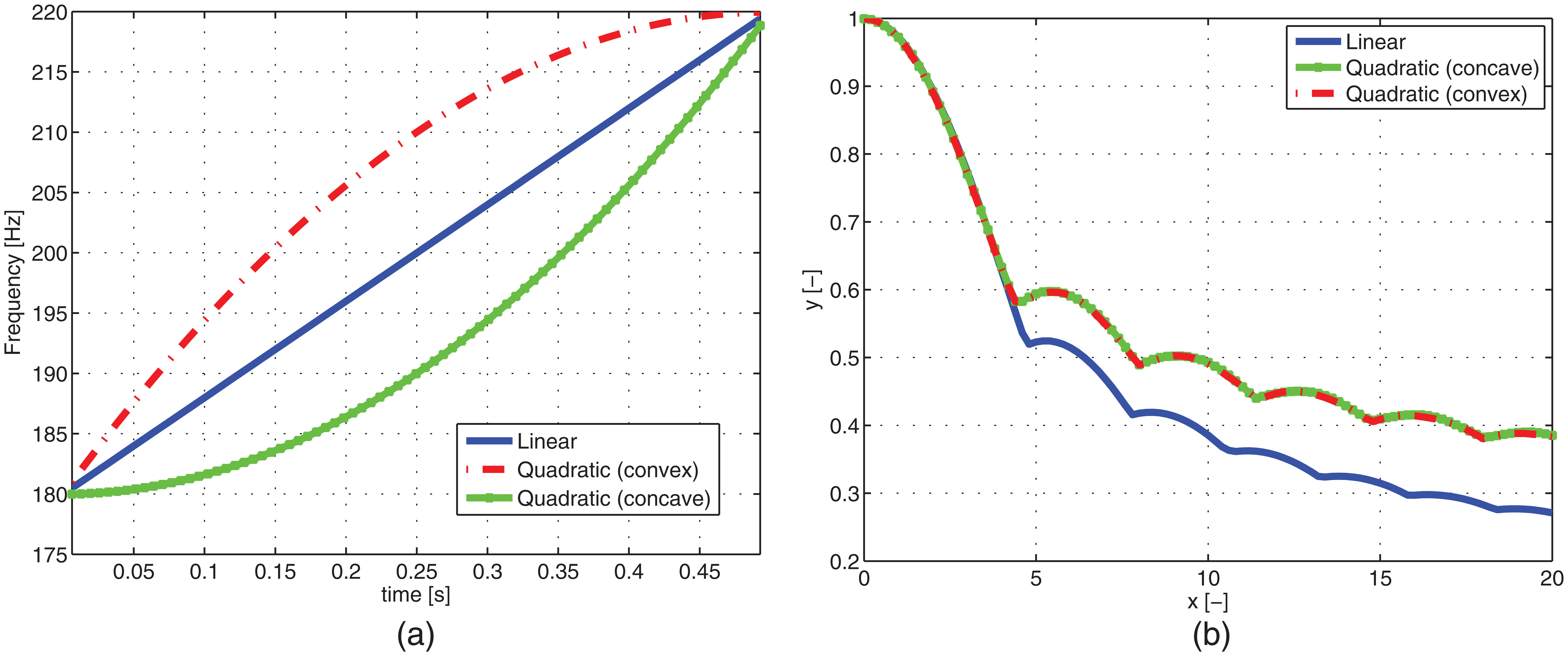
Influence of the frequency variation law of the analyzed signal in terms of amplitude: (a) frequency variation laws for the case x = 20 and (b) amplitude error for different smearing degrees using a rectangular window.

Figure 4(b) is analog to Figure 3, but it is computed considering the three different frequency variation laws and with the same initial and final frequencies. With reference to Figure 4(b), it can be noted that the amplitude error y for a particular window depends not only on the initial and final frequencies but also on the way in which the frequency sweeps from one value to the other. For all the frequency variation laws, the amplitudes are practically the same up to a value x = 4. This behavior can be justified considering that low values of smearing coefficient x refer to very flat curves; hence, the quadratic variations, concave and convex, have very low curvatures and the three curves are practically coincident. On the other hand, at high values of x the difference between the curves becomes more important: the quadratic curves continue to remain overlapped but diverge with respect to the linear case.

An alternative method for order tracking

This section discusses the principle on which the proposed algorithm is based. Furthermore, some of the most important aspects to consider when determining the amplitude of a certain harmonic using the DFT are studied in order to illustrate the capabilities and limitations of the proposed approach.

Algorithm principle

The autopower spectrum (APS) shows how the power of a signal is distributed in the frequency domain. ² The magnitude of the APS of a time trace $z(n)$ with its trend removed is equal to the square of the magnitude of the spectrum obtained with the DFT, that is

$$\mathrm{APS}(k)={\left[\frac{2A_w}{\sqrt{2}L}|\sum _{n=0}^{N-1}z(n)w(n)e^{-j2\pi \mathrm{kn}/N}|\right]}^2$$

(3)

where $A_w$ is the amplitude correction factor of the window $w(n)$ , $\sqrt{2}$ scales to the RMS value, 2 is due to the symmetry of FFT, N is the blocksize after zero padding, ² L is the original length of the block, and $n$ and $k$ are the indexes of the discrete time samples and the discrete frequency lines, respectively. Note that if zero padding is not used N = L.

The amplitude correction factor is constant for a particular window and can be calculated as ²

$$A_w=\frac{L}{\sum _{n=0}^{L-1}w(n)}$$

(4)

Parseval’s theorem ² implies that a mean square summation in the time domain is equivalent to a magnitude square summation in the frequency domain. Since, as well known, the RMS value of a signal ( $A_{\mathrm{RMS}}$ ) is the square root of the mean square summation in time domain, it yields

$$A_{\mathrm{RMS}}=\sqrt{\frac{L}{N}\frac{\sum _{k=0}^{N-1}\mathrm{APS}(k)}{B}}$$

(5)

where $B$ is the normalized equivalent noise bandwidth, which is a constant that depends on the window function used when computing the DFT. This constant can be calculated as ²

$$B=\frac{L\sum _{n=0}^{L-1}{w}^2(n)}{{[\sum _{n=0}^{L-1}w(n)]}^2}$$

(6)

Obviously, for a rectangular window $B=1$ . Hence, $A_{\mathrm{RMS}}$ is simply the root of the sum of squares of the component RMS values. Since Parseval’s theorem is valid also for sweeping sines, it is possible to compute the amplitude of the harmonic of interest from the information in the APS. This is the principle at the basis of the developed method.

Figure 5 is similar to Figure 2, but represents the APS. As stated above, an APS shows how the power of a signal is distributed in the frequency domain: it can be appreciated that the peak becomes wider as the frequency variation in the signal increases. Loosely speaking, it may be inferred that smearing does not affect the amount of the signal power but only causes a different spectral distribution. As a matter of fact, the summation of all the values in the APS, and therefore the area under the peak, remains constant as the smearing degree increases.

Figure 5.

Autopower spectrum.

Numerical investigations on the APS show that the area under the peak (for a signal with a single tone) remains constant even when changing the following:

• The amount of frequency variation in the signal;

• The frequency variation law;

• The sampling frequency (as long as Shannon’s sampling theorem ² is respected);

• The number of points used to compute the spectrum.

The fact that the area under the peak related to a certain tone in the APS remains constant as the parameters influencing smearing change serves as a starting point for the development of a method for the correction of the amplitude values obtained with the DFT. After computing the mentioned area $S$ through numerical integration (e.g. using the trapezoidal integration method), the final step is to determine the RMS value of the harmonic of interest; from equation (5), it follows that

$$A_{e,\mathrm{RMS}}=\sqrt{\frac{\mathrm{TS}}{B}}$$

(7)

Note that equation (7) yields the RMS value of the signal if the APS is scaled to the RMS value as defined in equation (3).

Aspects of DFT analysis considered during algorithm design

This section presents a series of considerations made during the design of the proposed approach regarding the characteristics of the analyzed signals and the input parameters of the DFT. This information will allow the reader to appreciate the capabilities and limitations of the method.

Effect of the spectrum frequency increment

It is worth noting that if the computation of the area was limited to a fixed number of spectral lines around the peak, for example, 5 as suggested in Brandt, ¹ the amplitude error would increase as the frequency increment of the spectrum $\mathrm{\Delta }f$ reduces: as shown in Figure 6(a) and (b), the whole area under the peak is described better by a fixed number of spectral lines (dashed lines with markers) when the frequency increment of the spectrum is larger. These APSs are computed for a stationary signal (x = 0) using a Hanning window with a frequency increment of 2 and 0.2 Hz, respectively. In the first case, the amplitude obtained is correct. Instead, the area described by five frequency lines around the peak with a frequency increment of 0.2 Hz yields an amplitude underestimation of about 50%.

Figure 6.

Effect of considering a fixed number of spectral lines, for example, 5, around the peak during the area calculation: (a) area described by a fixed number of spectral lines, Δf = 2 Hz; (b) area described by a fixed number of spectral lines, Δf = 0.2 Hz; and (c) amplitude errors due to smearing, Δf = 0.2 Hz.

Figure 6(c) is analog to Figure 3 but with a frequency increment of 0.2 Hz. The proposed approach gives the correct result (solid line) when all the APS spectral lines are considered, while, even for stationary signals, using the same method with a fixed number of spectral lines (dashed line) leads to an incorrect amplitude value. Moreover, the error committed also increases with the smearing degree. This is because the area under the APS peak is described better by a fixed number of spectral lines when the smearing degree is lower (see Figure 5).

There are basically two main reasons why it would be desirable to increase the resolution of the spectrum. The first one is computational efficiency: most of the commercial DFT algorithms require the blocksize to be a power of 2 for computational efficiency. ⁵ The second reason is leakage reduction: improving the resolution of the spectrum allows having frequency lines closer to the frequency of interest. ⁵

Consequently, the method was computed with the objective of considering the whole area under the peak relative to the order of interest after applying the DFT using zero padding (the implementation of the algorithm is detailed in section “Algorithm implementation”).

Choosing the window function

The proposed method is designed to apply the Hanning window to the signal before calculating the DFT: the choice of this window is due to the good trade-off between frequency resolution (intended as the capability of distinguishing two nearby frequencies) and leakage reduction. For a Hanning window, A_w = 2 and B = 1.5.

Figure 7 shows the APS of a signal composed of two closely spaced tones with frequencies of 200 and 205 Hz (amplitudes equal to 1). The frequency increment is 2 Hz (T = 0.5 s). The DFT was computed using two different window functions: Hanning (solid line with markers) and flattop (dashed line with markers). The APS obtained using a Hanning window gives the right value for the 200-Hz harmonic, that is, the squared RMS value of the sine. On the contrary, due to the fact that 205 Hz does not match a frequency line exactly (the closer ones are at 204 and 206 Hz), the power of that frequency component leaks out to nearby spectral lines which have values that are lower than the real one (leakage).

Figure 7.

Comparison of two different windows.

However, in the APS obtained using a flattop window, the two frequency components cannot be distinguished at all. This result clearly illustrates that stated in Brandt: ²

the flattop window, because of its large main-lobe width, should only be used when it is known that the spectrum does not contain any closely spaced tones. The Hanning window should, therefore, be used as a standard window since it provides a good compromise between amplitude accuracy and frequency resolution.

Furthermore, since a unique peak is visible in the APS computed with the flattop window, the algorithm is not able to separate the information of the two distinct harmonics.

Dealing with close orders

From the previous discussions, it is clear that the proposed approach cannot be used if the peak considered during the area computation is the result of two or more very close harmonics. The objective of this paragraph is to explore in what extent this is a limitation for the implementation of the algorithm.

A series of 1 s speed run-up tests are simulated, starting from 840 r/min, for different smearing degrees (using linear frequency variations). This is to evaluate a worst-case condition; in fact, it is well known that orders are closer in frequency at lower speeds. The proposed method is then implemented, exactly as it will be explained in section “Algorithm implementation” in order to determine the maximum value of the smearing degree that causes an error in the amplitude estimation of a particular order that is lower or equal than 10%. The analyzed signals contain the first five orders, each of them with a constant amplitude equal to 1.

Since the signal has more than one tone, it is necessary to limit the integration in equation (7) to the area under the APS peak that corresponds to the frequency of interest, excluding spectral lines where the energy of other frequency components may be present. In the next figures, the dashed lines indicate the portion of the APS considered for the area computation, while the solid lines with markers indicate a triangular surface used to recover part of the APS not considered due to the extraction process.

Figure 8(a) shows the APS of the signal when the speed at the end of the time-block is 1140 r/min (engine angular acceleration of 31 rad/s²). Five peaks are clearly visible. Note that the smearing effect increases with the order, yielding higher errors in the amplitude estimated with the DFT. Moreover, with this frequency variation, the peaks of the fourth and fifth orders become wide enough to start interacting with each other. Part of the energy of these two orders is smeared over the same frequency lines. Hence, the amplitudes of the peaks do not decrease smoothly as shown in Figure 5; instead, some irregularities are visible. However, the proposed approach retrieves the amplitudes of the first four orders exactly.

Figure 8.

Effect of different angular acceleration values on the APS: 31 rad/s²: (a) estimation of fourth-order amplitude with a negligible error and (b) 119 rad/s²: second-order amplitude estimated with an error lower than 10%.

In Figure 8(b), the angular acceleration is increased to 119 rad/s². With this frequency variation, the peaks for the last three orders are no longer distinguished. However, the amplitude of the first order is estimated exactly and the one of the second is computed with a 90% accuracy.

Table 1 presents the value of the maximum smearing degree that allows having an error lower than 10% for each order. The correspondent engine speed acceleration ( $\stackrel{·}{\omega }$ ) is also reported in the last column.

Table 1.

Maximum smearing degree for having an error lower than 10% with an initial speed of 840 r/min.

Order	x	$\stackrel{·}{\omega }$ (rad/s2)
1	55	346
2	38	119
3	36	75
4	32	50

It is worth mentioning that the highest smearing degree for the first order seen in the experimental data analyzed in section “Algorithm implementation” was about 7, thus meaning that the maximum value of x observed experimentally for each order was lower than the one reported in Table 1.

Furthermore, it is interesting noticing that in order to reach a smearing degree equal to the one yielding a 10% underestimation of the first-order amplitude, the car used during the experimental tests would need to have a longitudinal acceleration around 6 m/s².

Effect of signal amplitude change within the time-block

The method allows calculating the desired amplitude values when the energy of a particular order is smeared due to the signal frequency variation. If also the amplitude of the signal changes, it will be advisable to reduce the length of the time-block. Of course, this cannot be done arbitrarily since it would reduce the frequency resolution of the computed spectrum.

To illustrate the effect of a considerable change in the signal amplitude within the time-block on the results of the proposed method, a waveform of the first order, obtained applying a second-generation two-pole Vold-Kalman filter with a frequency bandwidth of 5 Hz to the experimental data analyzed in section “Algorithm implementation,” is used as a reference. A portion of the waveform, extracted around the transition between the idle phase and the beginning of the speed run-up, presents a considerable difference among its highest and lowest amplitudes (see Figure 9). Table 2 shows the absolute difference ( $\left|\Delta \right|$ ) between the amplitude estimated with the proposed technique and the value at the middle of the window ( $t_m$ ) for each of the signal portions presented in Figure 9 (along with a 0.5-s signal, two overlapped sub-portions of 0.3 s are indicated within rectangles). Note that modifying the size of the time-block in order to reduce the amplitude variation within the analyzed signal can considerably improve the results.

Figure 9.

Amplitude change within the time-block.

Table 2.

Estimated amplitude for each time-block.

Time-block	$t_m$ (s)	$\left|\Delta \right|$ (%)	$\Delta f$ (Hz)
(a) T = 0.5 s	0.75	39	2
(b) T = 0.3 s	0.65	3	3.33
(c) T = 0.3 s	0.85	6	3.33

In Table 2, the absolute difference ( $\left|\Delta \right|$ ) is presented as a percentage with respect to the amplitude of the signal.

Note that, according to the considerations made, the user can evaluate the quality of the results obtained by simply looking at the signal spectrum. Consequently, having this information helps with the setting of the parameter $T$ .

Algorithm implementation

The implementation of the novel method can be summarized in the next few steps:

1. Apply the STFT to the signal and compute the APS.

   For each time-block,

2. Identify the frequency of the order of interest from the speed measurements.

3. Extract the portion of the APS to be considered during the area computation.

4. Using the triangular approximation, compute the area to be added to the one calculated in the previous step.

5. Estimate the amplitude of the order with equation (7).

In the next paragraphs, the former tasks will be explained in detail. In particular, the aforementioned algorithm is applied to track the first order of a single mass flywheel speed signal. The experimental data (solid line in the top plot of Figure 10) were recorded during a speed run-up test carried out on a B-segment passenger car with first gear engaged. The vehicle is powered by a four-stroke two-cylinder engine mated to a five-speed manual transmission.

Figure 10.

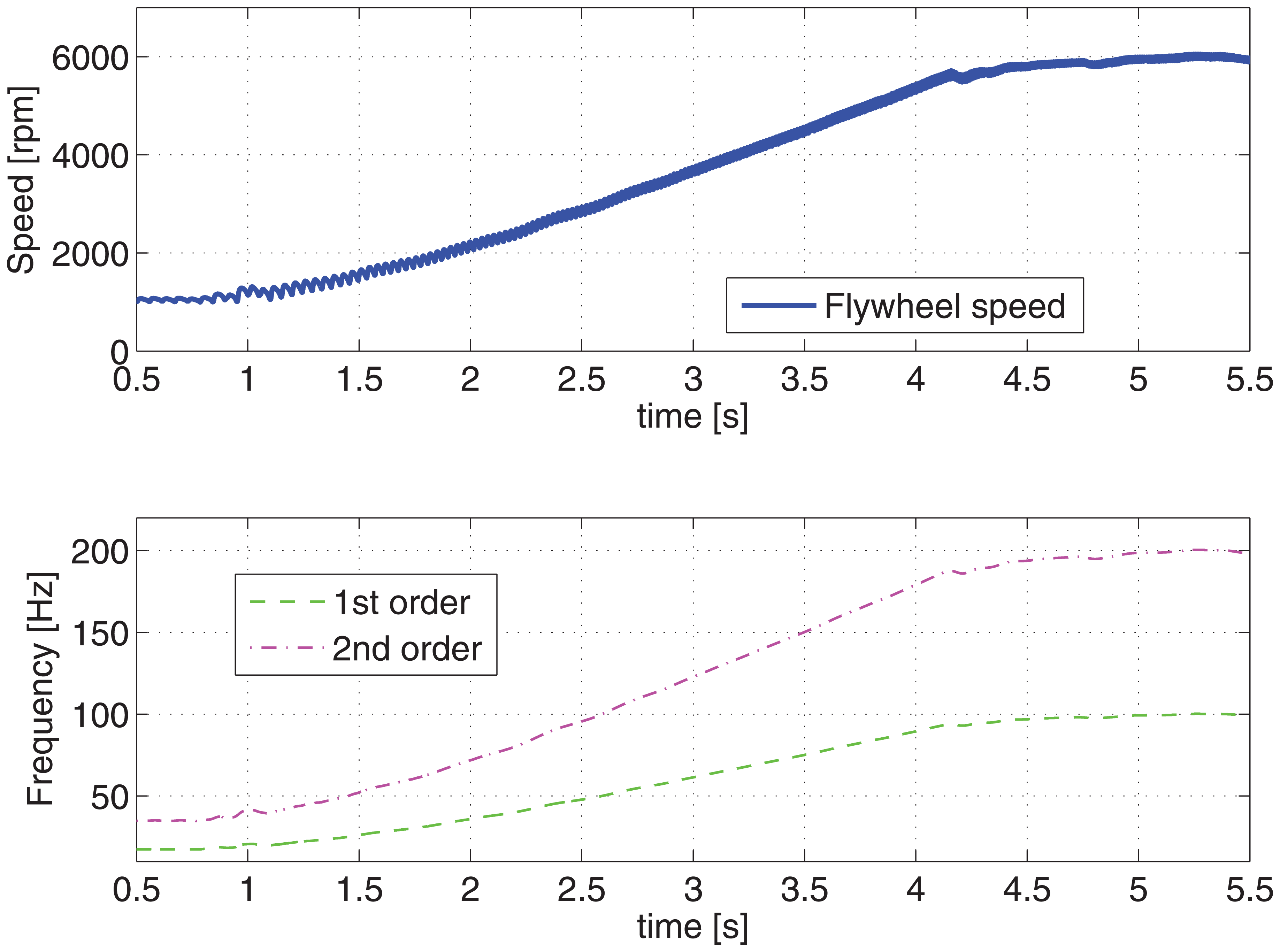
Flywheel speed and frequencies of the first two orders.

Computing the APS after applying the STFT

The first step is to divide the entire time history of the signal into different time-blocks (for this application, a 0.5-s window is used). Overlap may be employed to estimate more amplitude values (closely spaced in time) without reducing the blocksize. The DFT is implemented to signal portions of N points, N being the next power of 2 higher than or equal to 10 times L (zero padding is used). For each time-block, the APS is calculated using equation (3). Note that computing the APS by means of equation (3) implies removing the trend of the measured rotational speed.

Central spectral line identification

In order to extract the portion of each APS necessary to estimate the amplitude, the spectral line of the order of interest, named $o$ , must be identified. This identification process can be decomposed into two steps.

Step I

A first-attempt value of the order frequency $f_o$ is calculated from the filtered rotational speed ${\omega }_f$ (a 10-Hz low-pass digital filter is applied to the measured instantaneous angular speed) evaluated at the center of each time-block $\omega$

$$f_o=\frac{{\omega }_f}{2\pi }o$$

(8)

As an example, the estimated frequencies for the first two orders are shown in the lower part of Figure 10.

Step II

Search for the spectral line corresponding to the maximum amplitude of APS within a certain frequency range around $f_o$ . The information in the experimental spectrums obtained with the DFT allows inferring that the difference between the calculated frequency $f_o$ and the peak frequency grows with the engine speed. The proposed tolerance range $\Delta f_o$ allows handling this issue, that is, it increases with the engine speed and with order number. The tolerance range around the first attempt is

$$\Delta f_o=o(0.01\frac{{\omega }_f}{2\pi }+1)$$

(9)

Area under the peak extraction

After identifying the frequency of interest, the next fundamental step is to extract the portion of the APS that contains the entire area under the peak corresponding to the desired order, as required to compute the amplitude with equation (7). Again this task is divided into two steps.

Step I

A first attempt is to establish a tolerance range equal to half of the frequency of first order around the identified spectral line. This choice works well up to the fourth order of the experimental data analyzed, but can be optimized increasing the range with the order due to the effect of smearing.

Step II

There may be some spectral lines nearby the frequency of interest that should not be considered during the calculation of the area under the extracted APS portion. As discussed for the simulated signal in Figure 5, the amplitude on both sides of the peak in the APS should decrease (if there is no other frequency content apart from the order of interest and the amplitude remains constant within the time-block). Hence, the frequency bins on both sides of the peak where the amplitude increases with respect to the previous value are identified and the area computation is limited to the spectral lines around the peak that are between the two points that precede the identified frequency bins.

The identification of the spectral line where the amplitude starts to increase is applied for all points on both sides of the peak with an amplitude lower than a threshold, for example, half of the maximum value, since it was seen from the experimental data that for higher orders there may be some irregularities in the top portion of the peak that should not be excluded from the calculations.

Figure 11 illustrates this issue: the APS curve has two maxima. The APS portion extracted applying the identification process to all frequency lines with an amplitude lower than the peak value (solid line) is clearly smaller than the one obtained by taking into account only the spectral lines on both sides of the peak with an amplitude lower than half of the maximum value (solid line with markers). In fact, the amplitude estimated considering the smaller APS portion (threshold a = 100%) is about 29% lower than the mean value of the two methods used as reference, that is, Vold-Kalman filter (with a 5-Hz frequency bandwidth) and synchronous resampling (implemented using a sampling frequency of 360 points per revolution). The accuracy reaches 99.9% if the threshold is fixed to the 50% of the peak value.

Figure 11.

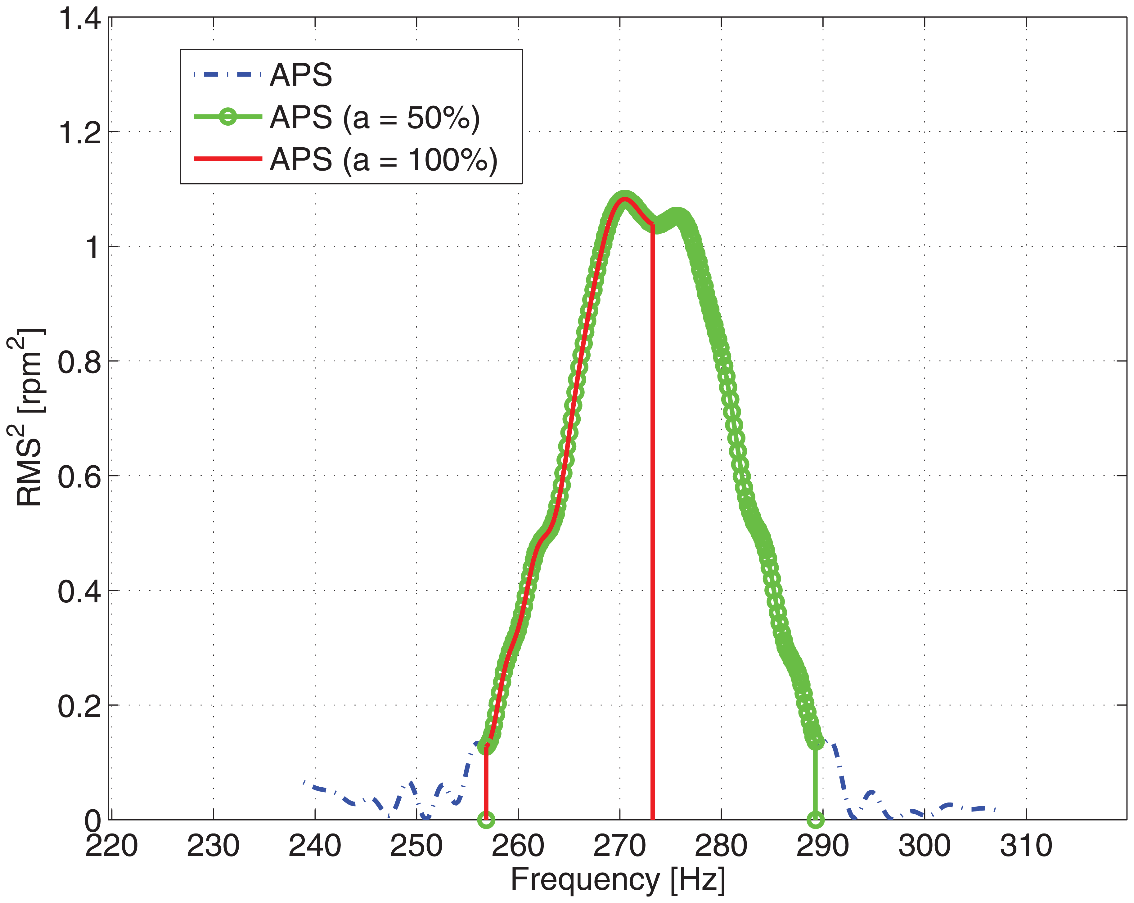
Irregularities in the top portion of the peak (fourth order) and identification of the spectral lines around the peak using two threshold values.

For example, the algorithm to identify the index ( $k_r$ ) of the last spectral line, on the right side of the APS peak and shown in Figure 11 for a = 50%, is as follows:

• $Require:AP{S}_r,N_r$

• $1:{\mathrm{Set\; k}}_{\mathrm{r}}={\mathrm{N}}_{\mathrm{r}}$

• $2:\mathbf{for}\mathrm{i}=1{\mathrm{to\; N}}_{\mathrm{r}}-1\mathbf{do}$

• $3:\mathbf{if}{k}_r=N_r\mathbf{do}$

• $4:\mathbf{if}{\mathrm{APS}}_{\mathrm{r}}\left(\mathrm{i}+1\right)>{\mathrm{APS}}_{\mathrm{r}}\left(\mathrm{i}\right)\&{\mathrm{APS}}_{\mathrm{r}}\left(\mathrm{i}+1\right)<0.5{\mathrm{APS}}_{\mathrm{p}}\mathbf{do}$

• $5:{\mathrm{k}}_{\mathrm{r}}=(\mathrm{i}+1)-2$

• $6:\mathbf{end\; if}$

• $7:\mathbf{end\; if}$

• $8:\mathbf{end\; for}$

where $\mathrm{AP}{S}_r$ is the APS portion on the right side of the peak and $N_r$ is its length in point number. $\mathrm{AP}{S}_p$ is the peak value.

Thanks to the methodology presented in this section for the extraction of the APS portion, for the case studied, good results can be achieved if the frequency components around the peaks related to the order of interest are not considered.

It is worth mentioning that other alternatives to the extraction process could be explored. Since the interference of close orders generates oscillations on the spectrum, as shown in Figure 8, a lower threshold should be set in order to avoid stopping the integral too early. For example, setting a = 10% when estimating the amplitude of the second order in Figure 8(b) yields y ≤ 1%. Since the left part of the peak does not seem to be mixed with other frequency components, another alternative could be estimating the area considered in equation (7) as twice the surface of the aforementioned section of the peak.

Increasing accuracy with linear extrapolation of APS

The explained extraction process is performed to avoid considering any spectral lines where the energy of other frequencies may be present. The APS portion considered in equation (7) is represented with a solid line in Figure 12, where a peak corresponding to the fourth order is shown.

Figure 12.

Area under the curve of the APS considered in the amplitude calculation for the fourth order.

The process of exclusion, discussed in the former section, implies that some parts of the lower area of the APS peak are not considered for the integral calculation. To take into account these regions, a triangular approximation is proposed. More specifically, the sides of the triangle (dashed lines with markers in Figure 12) are the vertical segment connecting the last considered point of the APS with the frequency axis, a portion of the linear extrapolation based on the last two points, and the resulting horizontal segment on the frequency axis.

The accuracy of the results adding the mentioned triangular surfaces generally increases. As an example, for the fourth order the amplitude estimations are 1% closer to the results of the Vold-Kalman method.

Comparison of different order tracking techniques

Figure 13 shows the comparison between the proposed method and other existing order tracking techniques. The results of applying the STFT to the original signal and after a synchronous resampling of the data (cyclic frequency of 360 points per revolution) are also shown for comparison. Furthermore, a second-generation two-pole Vold-Kalman filter with an adaptive frequency bandwidth based on the current angular speed at each instant (sample) of the signal, which leads to a 20% order bandwidth,^1,3,8 is applied to the data. Finally, the result of GOT with Gaussian windows of 50,000 points and an order bandwidth of 90% is also shown.

Figure 13.

Comparison between different order tracking methods (first order).

Figure 13 allows appreciating the validity of the developed method for order tracking: the results obtained with this approach are very close to other well-known techniques.

The running time of each order tracking method was measured using the same computer. The proposed approach is about 80% faster with respect to synchronous resampling and 29% slower than the Vold-Kalman filter. Since GOT was implemented using a different software (LabVIEW, whereas the others were applied using MATLAB), it is not included in the running time comparison.

The analysis of similar experimental tests executed at different gears allows noting that the smearing effect over the amplitudes calculated with the DFT decreases with the engaged gear in the manual transmission. For the signal analyzed in Figure 13 (a test in first gear), the mean difference between the first-order amplitudes calculated with an STFT and the explained technique is around 20%.

Figure 14 presents a spectrogram of the signal obtained with a regular STFT (0.5 s time-blocks with 90% overlap): there are some frequency components around the orders, especially at low speeds, that may cause difficulties in distinguishing between adjacent orders.

Figure 14.

Spectrogram of the angular speed during run-up test computed by means of STFT.

Moreover, since it is not clear to what extent these components are related to the frequencies of interest, considering more or less of this information (similarly to modifying the bandwidth of the mask in GOT or the Vold-Kalman filter) will affect the results.

For the Vold-Kalman filter, increasing the frequency bandwidth modifies the envelope and therefore changes the amplitude values extracted for a particular time/speed, as visible in Figure 15. Amplitude oscillations are evident for higher order bandwidths (e.g. 50%). Note that a narrower filter (5% order bandwidth) produces slowly varying orders, whereas a wider filter (20% order bandwidth) allows faster changes as function of the angular speed.

Figure 15.

Vold-Kalman filter with different bandwidths.

In the software used for the implementation of GOT, the elements of the Gabor coefficients matrix extracted for the reconstruction of the selected order waveform are identified using a mask with a fixed order bandwidth established from a visual inspection of a spectrogram similar to the one presented in Figure 14. The different bandwidths (using 50,000 points windows) modify the reconstructed waveforms, and therefore the computed envelopes, as shown in Figure 16.

Figure 16.

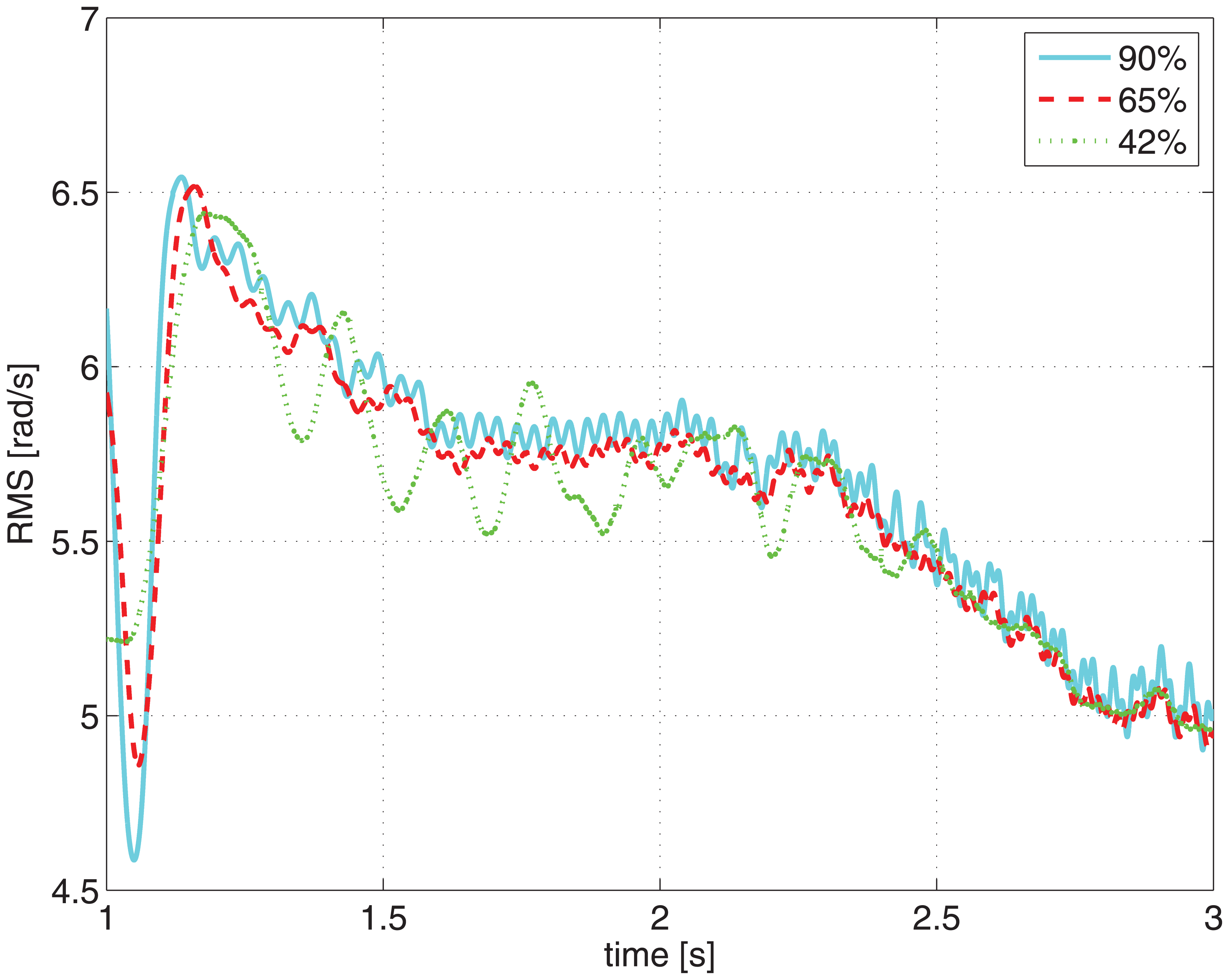
Gabor order tracking with different mask bandwidths.

The effect of the blocksize on the amplitudes estimated with the developed approach is presented in Figure 17: the amplitude of the first order is computed with a 50% overlap varying the windows temporal length. Increasing T reduces the capability of following fast changes in the order amplitude.

Figure 17.

Effect of the window length.

In addition, overlap may be employed to estimate more amplitude values (closely spaced in time) without reducing the blocksize. The increased time resolution can be appreciated in Figure 18.

Figure 18.

Increased time resolution with overlap.

Therefore, a proper combination of the two parameters can lead to accurate amplitude results together with an adequate time resolution.

Conclusion

In this article, a new STFT-based method for order tracking is presented, which uses information contained in the APS to compensate the spectral smearing; the result is an increased accuracy of the estimated order amplitudes.

Smearing may cause important errors when using STFT to estimate the amplitude of a signal whose frequency changes with time. For the analyzed case of a manual transmission in first gear during a speed run-up, STFT underestimates about 20% the amplitudes of the first order. Moreover, it has been shown that the estimation error due to smearing depends on the way in which the frequency varies from one value to the next and not only on the two extreme frequency values.

Conceptually, the proposed approach is based on the understanding that the energy of a harmonic signal is independent of its frequency variation in the observation window. The implementation of this idea implies an integration process in the APS to evaluate that energy, that is, the area under each peak.

For signals with rich frequency content, a method to limit the number of spectral lines around the peak considered during the integration process is proposed. If the calculation is restricted to a fixed number of spectral lines around the peak of the harmonic of interest, the amplitude error may increase with the smearing degree and with the frequency increment of the spectrum.

The effect of two input parameters of the algorithm is highlighted: increasing the blocksize reduces the capability of following fast changes in the order amplitude, whereas overlap may be employed to increase time resolution without reducing the blocksize.

The main limitation of the proposed approach is that it cannot be used for identifying the oscillation amplitude of very close and crossing orders. The case of close orders has been analyzed in detail: when the orders interact with each other, that is, part of their energy is smeared over the same frequency lines, the shape of the peaks is no longer smooth, but irregularities arise on the spectrum. From this point of view, the limits of application of this algorithm have been quantified in terms of maximum engine acceleration in order to avoid estimation errors over than 10% for the first four orders.

Considering the accuracy of the results, low use of computational resources, and ease of implementation, the proposed method proves a valid alternative to the currently used order tracking techniques, especially for the analysis of the vibrations due to internal combustion engine on passenger cars.