
Abstract
In this article, we describe the use of a new dynamic cubic nonlinear model, a new nonlinear subgrid-scale model, for simulating the cavitating flow around an NACA66 series hydrofoil. For comparison, the dynamic Smagorinsky model is also used. It is found that the dynamic cubic nonlinear model can capture the turbulence spectrum, while the dynamic Smagorinsky model fails. Both models reproduce the cavity growth/destabilization cycle, but the results of the dynamic cubic nonlinear model are much smoother. The re-entrant jet is clearly captured by the models, and it is shown that the re-entrant jet cuts the cavity into two parts. In general, the dynamic cubic nonlinear model provides improvement over the dynamic Smagorinsky model for the calculation of cavitating flow.
Introduction
Cavitation is an unsteady flow phenomenon that usually has a negative or even destructive effect on hydraulic machinery embodied in pressure pulsation, erosion, and noise.1,2 Cavitation occurs when the liquid pressure is lower than the saturated vapor pressure. In physical experiments, cavitation is produced by decreasing the pressure at the inlet or outlet of the flow field, leading to different types of cavitation that can be observed during this process. As the pressure decreases, an air cavity is stably attached to the surface of blades, followed by the development of cloud cavitation due to the destabilization of the cavity, resulting in the shedding of large vapor bubbles. Cloud cavitation is commonly associated with hydraulic machinery blades, and it has a highly dynamic flow pattern. 3 The intrinsic mechanism is often attributed to the re-entrant jet generated at the end of the cavity.4–6
In order to simulate the unsteady characteristics of cavitation through numerical calculation, it is usually assumed that the vapor and liquid are mixed and that they share the same velocity and pressure with a no-slip velocity condition between the two phases, as proposed by Kubota et al. 7 Based on this assumption, Transport-Based Equation Modeling (TEM) is widely used in cavitating flows. With this method, an additional advection equation is solved. Many cavitation models have been used for this framework. For example, Singhal et al. 8 developed the full cavitation model; Kunz et al. 9 proposed a three-species formulation to account for the liquid, vapor, and the non-condensable gas. Apart from the advection equation, the other aspects related to TEM are the solution strategy for the advection equation and the turbulence model. 10
As a solution strategy, Volume of Fluid (VOF) method is a good technique with the advantage of the ability to capture the cavity interface accurately. A brief review of different VOF models can be found in Roohi et al. 10 The application of VOF in various cavitating flows has been shown to be successful in tracking the cloud and super-cavitation cavities.10,11
For simulating turbulence, both Reynolds-averaged Navier–Stokes (RANS) and large eddy simulation (LES) models are widely used, although it seems that the results obtained with RANS modeling are not satisfactory without modification of the original formulations. For instance, Zhou and Wang 12 studied a two-dimensional (2D) hydrofoil and found that the standard re-normalization group (RNG) k-ε model could not capture the cavity shedding unless the turbulent viscosity was modified to account for cavitation.
The theoretical basis of LES modeling is its ability to capture large vortical structures including cloud cavitation. Liu et al. 13 used the Smagorinsky–Lilly model to study the cavitation on hydrofoil and successfully predicted the existence of the re-entrant jet; Ji et al. 14 used the wall-adapting local eddy viscosity (WALE) model and also reproduced the cavity shedding. Both models needed no further modification, showing an obvious advantage over the regular RANS models. However, the simulated pressure pulsation, which is an important aspect of the cavitation process, tended to fluctuate more than the experiment.14,15
A review of the literature shows that the LES models assume a linear relationship between the subgrid-scale (SGS) stress and the rate-of-strain, which may be the reason for the disagreement with experiment, as it has been figured out that the eigenvectors of the strain rate tensor and SGS stress tensor are not aligned but with a certain degree between each other in this linear relation.16,17 A more reasonable relation to use would be the nonlinear tensorial polynomial constitutive form, which combines SGS stress with strain rate and vorticity.
In order to examine the performance of nonlinear models in simulating cavitating flow, a new nonlinear SGS model is proposed to simulate the cavitation around a hydrofoil. The results are compared with the experimental data obtained by Leroux et al. 6 and with the numerical results of the dynamic Smagorinsky model (DSM).
Governing equations
LES modeling
In the LES model, a low-pass filter (in frequency) is applied to the Navier–Stokes equations to get the following formulations (in Cartesian coordinates)

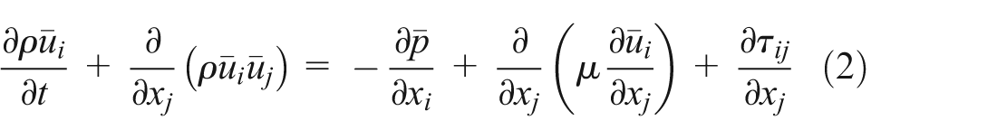
where the variables with a r bar over them represent the filtered quantities, u is the velocity, p is the pressure,


where

DSM
DSM is a linear eddy viscosity model. The Smagorinsky model can be expressed as

where
In order to dynamically calculate the model coefficient

where “∼” is the test-filtering operation and
where

Using equation (9) to provide an approximation to
The use of least squares minimization of the error is suggested by Lilly
19
for the calculation of the value of

It is well known that DSM suffers from numerical instability due to the large oscillation of the model coefficient. In this article, the eddy viscosity is bounded as

which means that the backscatter cannot be larger than the viscous dissipation (
Dynamic cubic nonlinear model
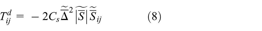
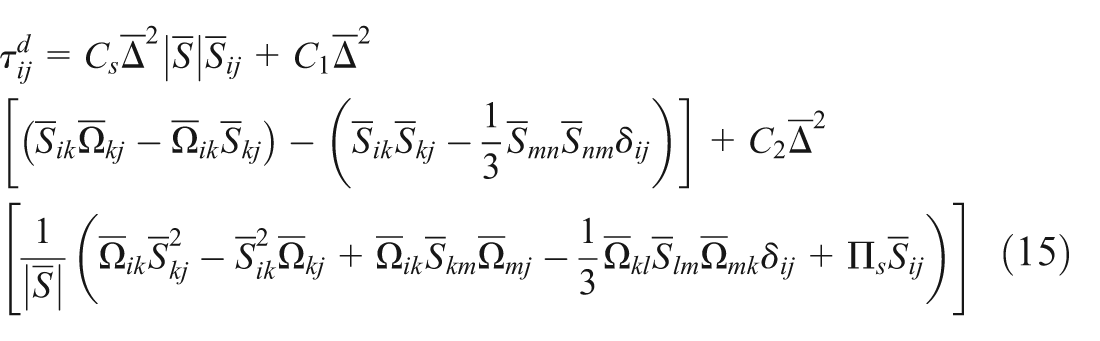
Kosovic 20 proposed applying the concepts of nonlinear models of different levels of complexity for Reynolds stress closures to SGS model as they have been extensively studied by researchers and are much more developed. Therefore, Shih et al.’s method 21 is applied for the construction of the new model. The general form of the new model can be written as follows

where

Adapting the above model to the simple shear flow, it can be shown that equation (13) does not stand. Comparing with the Kosovic model,
20
the term
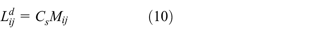
In order to dynamically calculate the three model coefficients (Cs, C 1, and C 2), the method proposed by Wang and Bergstrom 22 is applied. This is an extension of Germano’s method. The least square method is used

where


We named the dynamic cubic nonlinear model (DCNM) as the new model contains a cubic term. In order to guarantee the numerical stability and save computation resources, the coefficients in equation (16) are expressed explicitly with the volume average applied to both the numerator and denominator of each coefficient’s expression.
Two-phase modeling
As discussed above, TEM is used and the mixture model is considered in this article. In the mixture model, the fluids are treated as a combination of vapor and liquid, and an additional transport equation is written as
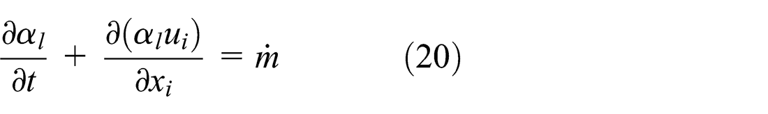
where


where
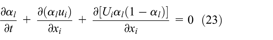
In OpenFOAM, 23 the VOF method is an improved version of CICSAM (Compressive Interface Capturing Scheme for Arbitrary Meshes) as follows
The compression velocity is calculated as

where

where

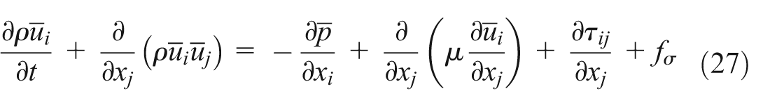
The surface tension is added to the momentum equation, and thus equation (2) is rewritten as
Numerical setup
The hydrofoil investigated in this study is an NACA66 series foil fixed in a square channel, with the chord length

Computational domain and boundary conditions.
The procedure proposed by Celik et al.
24
is used to examine whether the grid is in the asymptotic range. To resolve the near-wall characteristics,
The pressure coefficient is defined as
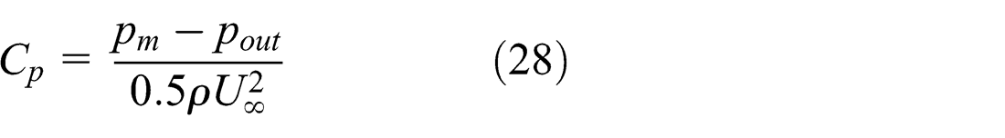
where

(a) Fine-grid convergence index and (b) extrapolated value comparing to the result of fine grid.
From the error bar shown in Figure 2(a), it can be seen that the fine-grid convergence index of the grid is small with an acceptable maximum error below 0.07. Figure 2(b) shows that the extrapolated value is close to that of the fine grid (with the number of grid elements equal to
Results and discussions
According to the experimental results reported by Leroux et al.,
6
when the cavitation number defined as
Pressure coefficient and cavity shedding frequency
Figure 3 shows a plot of the time-averaged value of

Comparison of the pressure coefficients along the suction side.
Due to the intrinsic relationship between cavitation and pressure, it is convenient to determine the cavity shedding frequency from the pressure signal. As was done in Ji et al.,
14
the power spectral density (PSD) is used in this article. Figure 4 shows the PSD profiles of two models, obtained in both cases by taking

PSD of DSM and DCNM at
Cavity growth/destabilization cycle
The cavity growth/destabilization cycle can be clearly illustrated by the numerical results, as shown in Figure 5. The iso-surface of the vapor volume fraction of 0.1 is used to show the cavity shape. It is observed that the cavity basically experiences three stages: (1) the cavity occurs at the leading edge and develops downstream; (2) when the cavity length is maximum, the cavity is cut into a partial cavity and a cloud cavitation by a pressure perturbation (shown in Figure 6); and (3) when the cloud cavitation reaches the trailing edge, the cavitation suddenly disappears (not shown). Both the models correctly reproduce the whole cycle compared with the experimental results. It should be noted that three-dimensional characteristics are shown in the spanwise direction, which would probably lead to the overestimation of the shedding frequency due to the reduced span width used in the calculations.

Cavity evolution in one cycle (time interval between two images: numerical data, 0.05 s; experimental data, 0.08 s): (a) DSM, (b) DCNM and (c) experiment.

Comparison of instantaneous pressure at
Three stages can be reflected in the temporal pressure signal on the suction side of the hydrofoil. Figure 6 shows a comparison of instantaneous pressure signals at
At stage 2, the cavity shedding is attributed to the re-entrant flow generated at the end of the cavity.4–6
Figure 7 shows the velocity vector field around the foil at

Predicted re-entrant flow on the suction side: (a) DSM and (b) DCNM.
Model coefficients and SGS dissipation
From the above analysis, it is found that the instantaneous pressure of DCNM is smoother than the DSM’s. The underlying reason can be attributed to the model behavior during the calculation. The model coefficient is a representative quantity which will vary during the calculation. Figure 8 shows the instantaneous non-dimensional model coefficient, which is defined as

Comparison of the instantaneous non-dimensional model coefficient at
As can be seen, the fluctuation of the model coefficient in DSM is much larger than in DCNM. This is a good indication that the pressure field calculated by DSM experiences more fluctuation.
Another index quantity is the non-dimensional SGS turbulent kinetic energy (TKE) production, which is defined as

Comparison of the instantaneous non-dimensional SGS TKE production at
Conclusion
In this article, we present the use of a linear model DSM and the new nonlinear model DCNM for the calculation of cavitating flow around an NACA66 series hydrofoil and the simulation results are compared with the experimental data. For both models, the cavity shedding frequency is overestimated, but the reason is still not clear. It is suspected that the reduced span width in the simulation may affect the shedding frequency as the cavitating flow shows three-dimensional characteristics. From the PSD analysis, it is found that DCNM can capture the turbulence spectrum while DSM fails to do so. The cavity growth/destabilization cycle, simulated by both models, duplicates the experimental data with little discrepancy.
Further investigation is done to explore the instantaneous pressure on the suction side. The results of DCNM are much smoother than in DSM, and this phenomenon may explain why DSM fails to capture the turbulence spectrum. Additionally, the re-entrant jet which cut the cavity into two parts is captured by the models. The instantaneous model coefficients and SGS TKE production are studied to reveal the underlying reason why DCNM predicts smoother pressure profile. It is found that both the model coefficient fluctuation and SGS TKE production are much larger for DSM. Additionally, significant backscatter of DSM is observed, which will affect the large-scale motions. Under these conditions, the pressure field is influenced in DSM, resulting in much fluctuation of the instantaneous pressure. In general, the nonlinear model does improve the ability to capture the turbulence, while it should be noted that the cavity shedding frequency is turbulence model independent. Further improvements of the calculation may focus on the cavitation model.
Footnotes
Academic Editor: Moran Wang
Declaration of conflicting interests
The author(s) declared no potential conflicts of interest with respect to the research, authorship, and/or publication of this article.
Funding
The author(s) disclosed receipt of the following financial support for the research, authorship, and/or publication of this article: The authors would like to acknowledge the financial support given by the Ministry of Education, Science and Technology Project (Grant No. 113010A), the Research Fund for the Doctoral Program of Higher Education of China (Grant No. 20130008110047), and the National Natural Science Foundation of China (Grant No. 51209206).