Fractional electrical circuits

Abstract

We study three different types of electrical circuit equations using fractional calculus and various definitions of fractional derivative therein. Using plotting tools, we compare different types of solutions of each equation among themselves as well as with its classical solution.

Introduction

Fractional calculus has seen many advancements over the past years and we find that many classical physics models are today being analysed using fractional differential equations. The theory and applications on such analysis can be found in several studies.^1–3

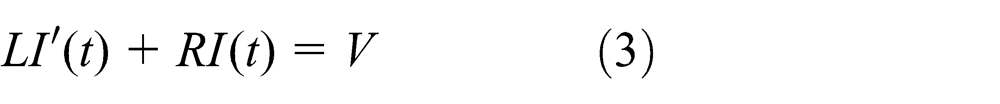
Here, we cover the basic equations of electric circuits involving resistors, capacitors and inductors. We analyse the following equations for three different types of circuits ⁴

$$I″(t)+\frac{1}{\mathrm{LC}}I(t)=0$$

(1)

$$\mathrm{CV}\prime (t)+\frac{1}{R}V(t)=0$$

(2)

$$\mathrm{LI}\prime (t)+\mathrm{RI}(t)=V$$

(3)

where $I(t)$ is the current in the circuit at time t, L is the inductance, C is the capacitance, R is the resistance and V is the voltage drop across the circuit. Equation (1) represents the LC (inductor–capacitor) circuit, equation (2) represents RC (resistor–capacitor) circuit and equation (3) represents LR (inductor-resistor) circuit. Some preliminary numerical results for RLC circuits are presented in Atangana and Nieto ⁵ and some extensions to fractional electric circuits in Atangana and Alkahtani. ⁶ For a more detailed analysis of fractional circuits, we refer the reader to Kaczorek ⁷ and the monograph. ⁸

We aim to solve equations (1)–(3) using fractional calculus and compare the results with classical solutions.

Preliminary results

While using fractional calculus, one has many choices for definitions of fractional integral as well as fractional derivative. Since we want to analyse the electric circuit differential equations using more than one type of fractional derivative, we consider the following approaches for the same, where the order of differentiation is always positive.

Definition 1

For a function f given on interval $[a,b]$ , the Riemann–Liouville fractional-order derivative of order $\alpha (n-1<\alpha \le n)$ of $f$ is defined by ⁹

$$D_a^{\alpha }f(t)=\frac{1}{\Gamma (n-\alpha )}{\left(\frac{d}{\mathrm{dt}}\right)}^n\underset{a}{\overset{t}{\int }}{(t-s)}^{-\alpha +n-1}f(s)\mathrm{ds}$$

provided the right-hand side is defined for a.e. t.

For example, $f\in L^1(a,b)$ implies that the Riemann–Liouville fractional derivative is well defined for f.

We define $A{C}^n([a,b])$ as a space of functions f such that f is absolutely continuous.

Definition 2

Let $f\in A{C}^n([a,b])$ . The Caputo fractional-order derivative of $f$ , order $\alpha (n-1<\alpha \le n)$ , is defined by ⁹

$${(}^c{D}_a^{\alpha }f)(t)=\frac{1}{\Gamma (n-\alpha )}\underset{a}{\overset{t}{\int }}{(t-s)}^{n-\alpha -1}{f}^{(n)}(s)\mathrm{ds}$$

Definition 3

Let $f\in A{C}^n([a,b])$ The Caputo–Fabrizio fractional-order derivative of $f$ , order $\alpha (0<\alpha \le 1)$ , is defined by ¹⁰

$${}^{\mathrm{CF}}{D}_a^{\alpha }f(t)=\frac{(2-\alpha )M(\alpha )}{2(1-\alpha )}\underset{a}{\overset{t}{\int }}\exp (-\frac{\alpha }{1-\alpha }(t-s))f\prime (s)\mathrm{ds}$$

The Caputo–Fabrizio fractional integral was previously introduced by Caputo and Fabrizio. ¹¹

Now, we present the generalized Mittag–Leffler function denoted by $E_{\alpha ,\beta }$ and defined as

$$E_{\alpha ,\beta }(z)≔\sum _{k=0}^{\infty }\frac{z^k}{\Gamma (k\alpha +\beta )}$$

Also

$$E_{\alpha ,\beta }(z)=\frac{1}{2\pi i}\underset{\Upsilon }{\int }\frac{{\lambda }^{\alpha -\beta }{e}^{\lambda }}{{\lambda }^{\alpha }-z}d\lambda$$

where $\Upsilon$ is a contour, which starts and ends at $-\infty$ and encircles the disc $\left|\lambda \right|\le {\left|z\right|}^{1/\alpha }$ counterclockwise.

Lemma 1

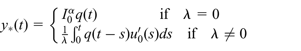
Let $\alpha >0,n=\lceil \alpha \rceil$ and $\lambda \in \mathbb{R}$ . The solution of the initial value problem ³

$$\{\begin{array}{c}\hfill {}^{c}D{}^{\alpha }y(t)=\lambda y(t)+q(t)\hfill \\ \multicolumn{1}{c}{y^{(k)}(0)y_k,k=0,1,\dots ,n-1}\end{array}$$

(4)

where $q\in C[0,b]$ is a given function and can be expressed in the form

$$y(t)=\sum _{k=0}^{n-1}{y}_k{u}_k(t)+y_{*}(t)$$

with

$$y_{*}(t)=\{\begin{array}{c}\hfill I_0^{\alpha }q(t)\mathrm{if}\lambda =0\hfill \\ \multicolumn{1}{c}{\frac{1}{\lambda }{\int }_0^{t}q(t-s)u{\prime }_0(s)\mathrm{ds}\mathrm{if}\lambda \ne 0}\end{array}$$

where $u_k(t)=I_0^k{e}_{\alpha }(t),k=0,1,\dots ,n-1$ and $e_{\alpha }(t)≔E_{\alpha }(\lambda t^{\alpha })$

Remark 1

In the case $0<\alpha <1$ , we can rewrite the solution of problem (4) in the form

$$y(t)=y(0)E_{\alpha }(\lambda t^{\alpha })+\alpha \underset{0}{\overset{t}{\int }}q(t-s)s^{\alpha -1}{E\prime }_{\alpha }(\lambda s^{\alpha })\mathrm{ds}$$

Lemma 2

For a differentiable function f defined on $[a,b]$ , we can relate its Riemann–Liouville and Caputo fractional-order derivatives as follows

$$D_a^{\alpha }(f(t)-\sum _{k=0}^{n-1}\frac{t^k}{\Gamma (k+1)}{f}^{(k)}(0^{+})){=}^c{D}_a^{\alpha }f(t)$$

where $\alpha \in {\mathbb{R}}_{+}$ and $n-1<\alpha \le n$ .

Lemma 3

Let $0<\alpha <1$ . Then, the unique solution of the following initial value problem ¹⁰

$${}^{\mathrm{CF}}{D}^{\alpha }f(t)=\sigma (t),t\ge 0$$

with $f(0)=f_0\in \mathbb{R}$ is given by

$$f(t)=f_0+a_{\alpha }(\sigma (t)-\sigma (0))+b_{\alpha }{I}^1\sigma (t),t\ge 0$$

where $I^1\sigma$ denotes a primitive of $\sigma$ and

$$a_{\alpha }=\frac{2(1-\alpha )}{(2-\alpha )M(\alpha )},b_{\alpha }=\frac{2\alpha }{(2-\alpha )M(\alpha )}$$

RLC circuits

In this section, we apply various approaches of fractional calculus to equations (1)–(3) and obtain some results of comparing their solutions with the corresponding classical solutions.

LC circuit

Only charged capacitor and inductor are present in the circuit and its differential equation is given as follows

$$I″(t)+\frac{1}{\mathrm{LC}}I(t)=0$$

(5)

with $I(0)=I_0$ and $I\prime (0)=0$ . We will represent $1/\mathrm{LC}$ as ${\omega }_0^2$ here onwards. The classical solution of equation (5) is

$$I(t)=I_0\cos ({\omega }_{0}t)$$

(6)

Now, to analyse equation (5) using fractional calculus, we replace $I″(t)$ by $D^{\alpha }I(t)$ (Riemann–Liouville), ${}^c{D}^{\alpha }I(t)$ (Caputo) and ${}^{\mathrm{CF}}{D}^{\alpha }I(t)$ (Caputo–Fabrizio) derivatives where $\alpha \in (1,2)$ .

Riemann–Liouville derivative

Now, equation (5) becomes

$$D^{\alpha }I(t)+{\omega }_0^{2}I(t)=0$$

(7)

Using Lemmas 1 and 2, the solution of equation (7) is given by

$$\begin{array}{c}\multicolumn{1}{c}{I(t)=I_0{E}_{\alpha }(-{\omega }_0^2{t}^{\alpha })+\frac{I_0}{{\omega }_0^2\Gamma (1-\alpha )}}\\ \multicolumn{1}{c}{\underset{0}{\overset{t}{\int }}{(t-s)}^{-\alpha }{s}^{\alpha -1}E{\prime }_{\alpha }(-{\omega }_0^2{s}^{\alpha })\mathrm{ds}}\end{array}$$

(8)

Caputo derivative

Now, equation (5) becomes

$${}^c{D}^{\alpha }I(t)+{\omega }_0^{2}I(t)=0$$

(9)

Using Lemma 1, the solution of equation (9) is given by

$$I(t)=I_0{E}_{\alpha }(-{\omega }_0^2{t}^{\alpha })$$

(10)

Caputo–Fabrizio derivative

Now, equation (5) becomes

$${}^{\mathrm{CF}}{D}^{\alpha }I(t)+{\omega }_0^{2}I(t)=0$$

(11)

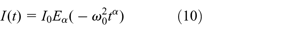
Using Lemma 3, the solution of equation (11) is given by

$$I(t)=I_0{e}^{\frac{p}{2}t}[\left(\frac{q-p}{2q}\right)e^{\frac{q}{2}t}+\left(\frac{p+q}{2q}\right)e^{-\frac{q}{2}t}]$$

(12)

where $p=(1-\alpha ){\omega }_0^2$ and $q=\sqrt{{[(1-\alpha ){\omega }_0^2]}^2-4\alpha {\omega }_0^2}$ .

Graphical comparison

Figure 1 shows the plots for equations (6), (8), (10) and (12). As it can be clearly seen, for $\alpha =1.5$ , all three fractional derivative graphs behave similarly and show damped oscillation eventually reaching to 0. Whereas the classical approach graph represents a simple harmonic oscillation (cosine curve). But when we take $\alpha =1.999$ (Figure 2), classical, Riemann–Liouville and Caputo derivative graphs overlap each other representing the harmonic oscillation in the values of current as time progresses. Even in this case, the Caputo–Fabrizio approach shows damping and behaves very differently from other graphs.

Figure 1.

Current versus time graph ( $L=1,C=1,I_0=0.01$ and $\alpha =1.5$ ).

Figure 2.

Current versus time graph ( $L=1,C=1,I_0=0.01$ and $\alpha =1.999$ ).

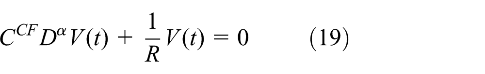
RC circuit

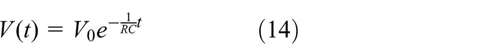
Only charged capacitor and resistor are present in the circuit and its differential equation is given as follows

$$\mathrm{CV}\prime (t)+\frac{1}{R}V(t)=0$$

(13)

with $V(0)=V_0$ . The classical solution of equation (13) is

$$V(t)=V_0{e}^{-\frac{1}{\mathrm{RC}}t}$$

(14)

Now, to analyse equation (13) using fractional calculus, we replace $V\prime (t)$ by $D^{\alpha }V(t)$ (Riemann–Liouville), ${}^c{D}^{\alpha }V(t)$ (Caputo) and ${}^{\mathrm{CF}}{D}^{\alpha }V(t)$ (Caputo–Fabrizio) derivatives where $\alpha \in (0,1]$

Riemann–Liouville derivative

Now, equation (13) becomes

$$C{D}^{\alpha }V(t)+\frac{1}{R}V(t)=0$$

(15)

Using Lemmas 1 and 2, the solution of equation (15) is given by

$$\begin{array}{c}\multicolumn{1}{c}{V(t)=V_0{E}_{\alpha }(-\frac{1}{\mathrm{RC}}{t}^{\alpha })-\frac{V_0\alpha }{\Gamma (1-\alpha )}}\\ \multicolumn{1}{c}{\underset{0}{\overset{t}{\int }}{(t-s)}^{-\alpha }{s}^{\alpha -1}E{\prime }_{\alpha }(-\frac{1}{\mathrm{RC}}{s}^{\alpha })\mathrm{ds}}\end{array}$$

(16)

Caputo derivative

Now, equation (13) becomes

$$C^c{D}^{\alpha }V(t)+\frac{1}{R}V(t)=0$$

(17)

Using Lemma 1, the solution of equation (17) is given by

$$V(t)=V_0{E}_{\alpha }(-\frac{1}{\mathrm{RC}}{t}^{\alpha })$$

(18)

Caputo–Fabrizio derivative

Now, equation (13) becomes

$$C^{\mathrm{CF}}{D}^{\alpha }V(t)+\frac{1}{R}V(t)=0$$

(19)

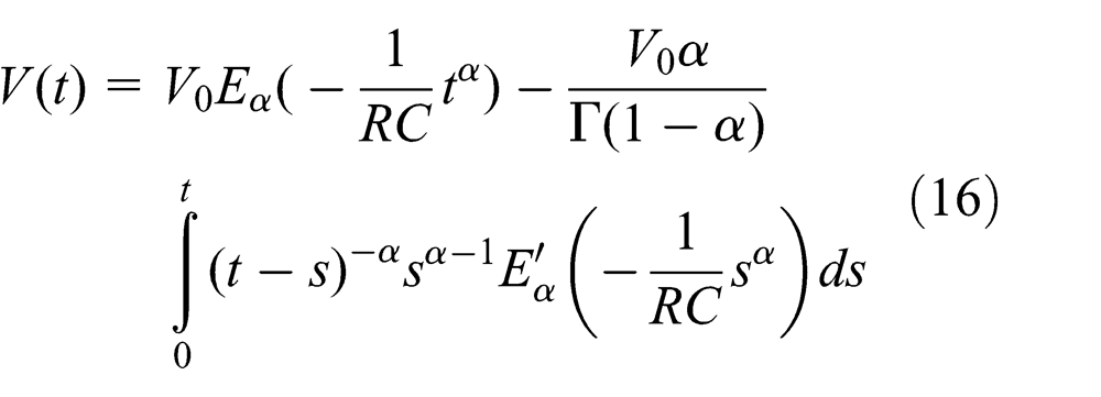
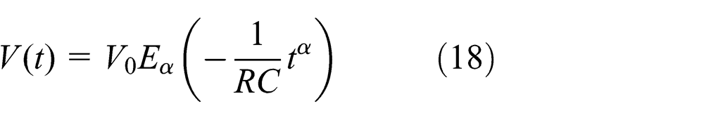
Using Lemma 3, the solution of equation (19) is given by

$$V(t)=V_0{e}^{-\frac{2\alpha }{2\mathrm{RC}+2(1-\alpha )}t}$$

(20)

Graphical comparison

Figure 3 shows the plots for equations (14), (16), (18) and (20). As it can be clearly seen, for $\alpha =0.5$ , classical and Caputo–Fabrizio fractional derivative graphs behave similarly and eventually reaching to 0. Whereas the Riemann–Liouville and Caputo fractional derivative graphs start similarly like the previous two, but later go to negative infinity as time moves forward. But when we take $\alpha =0.999$ (Figure 4), classical, Riemann–Liouville, Caputo and Caputo–Fabrizio derivative graphs overlap each other representing the simple decay of voltage in the circuit as time progresses. Even in this case, the initial value for Riemann–Liouville does not coincide with $V_0$ due to the presence of 1/t in its formula.

Figure 3.

Voltage versus time graph ( $C=1,R=10,V_0=20$ and $\alpha =0.5$ ).

Figure 4.

Voltage versus time graph ( $C=1,R=10,V_0=20$ and $\alpha =0.999$ ).

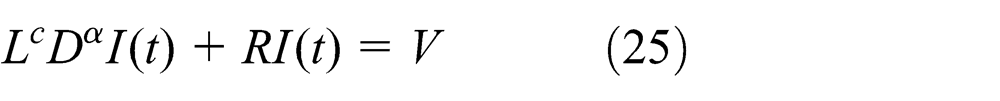
RL circuit

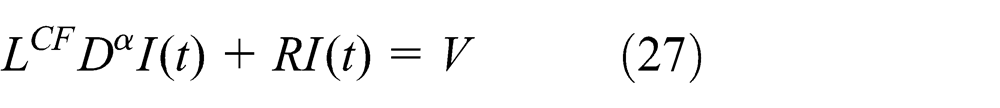
Only resistor, inductor and a non-variant voltage source are present in the circuit and its differential equation is given as follows

$$\mathrm{LI}\prime (t)+\mathrm{RI}(t)=V$$

(21)

with $I(0)=I_0$ and $V$ is the constant voltage source. The classical solution of equation (21) is

$$I(t)=[I_0-\frac{\mathrm{VL}}{R}]e^{-\frac{R}{L}t}+\frac{\mathrm{VL}}{R}$$

(22)

Now, to analyse equation (21) using fractional calculus, we replace $I\prime (t)$ by $D^{\alpha }I(t)$ (Riemann–Liouville), ${}^c{D}^{\alpha }I(t)$ (Caputo) and ${}^{\mathrm{CF}}{D}^{\alpha }I(t)$ (Caputo–Fabrizio) derivatives where $\alpha \in (0,1]$ .

Riemann–Liouville derivative

Now, equation (21) becomes

$$L{D}^{\alpha }I(t)+\mathrm{RI}(t)=V$$

(23)

Using Lemmas 1 and 2, the solution of equation (23) is given by

$$\begin{array}{c}\multicolumn{1}{c}{I(t)=I_0{E}_{\alpha }(-\frac{R}{L}{t}^{\alpha })}\\ \multicolumn{1}{c}{+\alpha \underset{0}{\overset{t}{\int }}[\frac{V}{L}-\frac{I_0{(t-s)}^{-\alpha }}{\Gamma (1-\alpha )}]s^{\alpha -1}E{\prime }_{\alpha }(-\frac{R}{L}{s}^{\alpha })\mathrm{ds}}\end{array}$$

(24)

Caputo derivative

Now, equation (21) becomes

$$L^c{D}^{\alpha }I(t)+\mathrm{RI}(t)=V$$

(25)

Using Lemma 1, the solution of equation (25) is given by

$$I(t)=[I_0-\frac{\alpha V}{R}]E_{\alpha }(-\frac{R}{L}{t}^{\alpha })+\frac{\alpha V}{R}$$

(26)

Caputo–Fabrizio derivative

Now, equation (21) becomes

$$L^{\mathrm{CF}}{D}^{\alpha }I(t)+\mathrm{RI}(t)=V$$

(27)

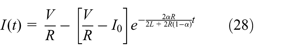
Using Lemma 3, the solution of equation (27) is given by

$$I(t)=\frac{V}{R}-[\frac{V}{R}-I_0]e^{-\frac{2\alpha R}{2L+2R(1-\alpha )}t}$$

(28)

Graphical comparison

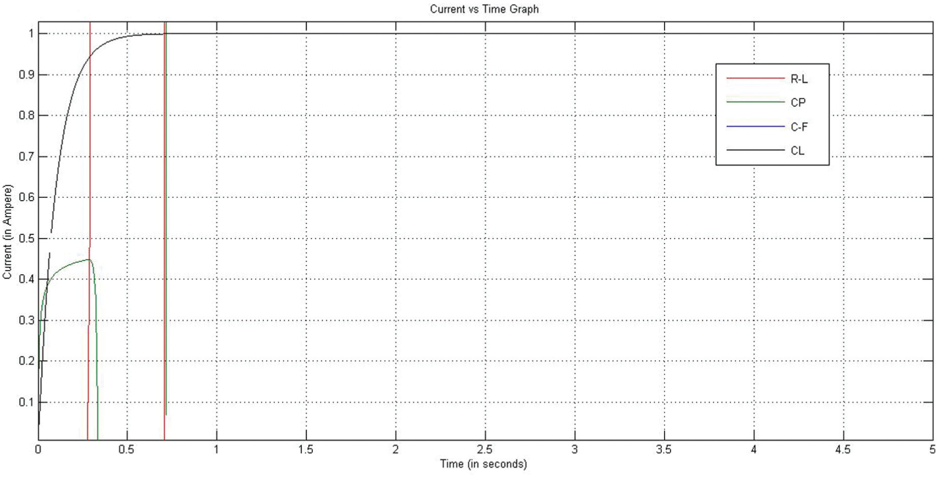
Figure 5 shows the plots for equations (22), (24), (26) and (28). As it can be clearly seen, for $\alpha =0.5$ , none of the four graphs shows any similarity in their behaviours. All the three fractional derivative graphs show varied divergence from the classical approach graph sometimes tending to positive/negative infinity. But when we take $\alpha =0.999$ (Figure 6), classical and Caputo–Fabrizio derivative graphs overlap each other representing exponential increase and then a steady state for the values of current as time progresses. The Caputo fractional derivative graphs coincide with the classical one but diverges to very large positive values as time progresses whereas the Riemann–Liouville graph shows no similarity at all.

Figure 5.

Current versus time graph ( $L=1,R=10,V=10,I_0=0.01$ and $\alpha =0.5$ ).

Figure 6.

Current versus time graph ( $L=1,R=10,V=10,I_0=0.01$ and $\alpha =0.999$ ).

Conclusion

We have applied the fractional derivative definitions and concepts on electrical circuit equations and compared them with their classical counterparts. As observed after studying the comparison graphs, we can state that fractional calculus acts as a generalization to the classical calculus. Such analysis can be further applied to other physical models to develop a better understanding of use of fractional calculus in real-life problems.

References

1.
MainardiF. Fractional calculus: some basic problems in continuum and statistical mechanics. In: CarpinteriAMainardiF (eds) Fractals and fractional calculus in continuum mechanics. Wien: Springer-Verlag, 1997, pp.291–348.
2.
AbbasSBenchohraMN’GuérékataGM. Topics in fractional differential equations. New York: Springer, 2012.
3.
DiethelmK. The analysis of fractional differential equations: an application-oriented exposition using differential operators of Caputo type, vol. 2004 (Lecture Notes in Mathematics). Berlin: Springer-Verlag, 2010.
AtanganaANietoJJ. Numerical solution for the model of RLC circuit via the fractional derivative without singular kernel. Adv Mech Eng. Epub ahead of print 29 October 2015. DOI: 10.1177/1687814015613758.
6.
AtanganaAAlkahtaniBST. Extension of the resistance, inductance, capacitance electrical circuit to fractional derivative without singular kernel. Adv Mech Eng. Epub ahead of print 26 June 2015. DOI: 10.1177/1687814015591937.
7.
KaczorekT. Positive electrical circuits and their reachability. Arch Elect Eng2011; 60: 283–301.
8.
KaczorekTRogowskiK. Fractional linear systems and electrical circuits. London: Springer, 2007.
9.
KilbasAASrivastavaHMTrujilloJJ. Theory and applications of fractional differential equations, vol. 204 (North-Holland Mathematics Studies). Amsterdam: Elsevier, 2006.
10.
LosadaJNietoJJ. Properties of a new fractional derivative without singular kernel. Progr Fract Differ Appl2015; 1: 87–92.
11.
CaputoMFabrizioM. A new definition of fractional derivative without singular kernel. Progr Fract Differ Appl2015; 1: 73–85.