Unsteady flow simulations of Pelton turbine at different rotational speeds

Abstract

This article presents numerical simulations of a small Pelton turbine suitable for desalination system. A commercial flow solver was adopted to resolve difficulties in the numerical simulation for Pelton turbine such as the relative motion of the turbine runner to the injector and two-phase flow of water and air. To decrease the numerical diffusion of the water jet, a new topology with only hexagonal mesh was suggested for the computational mesh around the complex geometry of a bucket. The predicted flow coefficient, net head coefficient, and overall efficiency showed a good agreement with the experimental data. Based on the validation of the numerical results, the pattern of wet area on the bucket inner surface has been analyzed at different rotational speeds, and an attempt to find the connection between rotational speeds, torque, and efficiency has been made.

Introduction

Desalination system using reverse osmosis (RO) process is generally being used for drinking water purification due to lower cost than other methods. RO uses a semi-permeable membrane for water purification but is slightly different from a traditional filtration method. High pressure larger than osmotic pressure is applied in RO so that the pure water stays on the pressurized side and the pure salt passes through the membrane. Consequently, RO process produces the pure water with high pressure as a byproduct. To increase the overall efficiency of desalination system, this high pressurized water can be used as a hydraulic energy source.

Pelton turbine is suitable to generate electric power efficiently using a relatively small amount of high pressurized water in the desalination system to recover renewable energy. Pelton turbine is an impulse-type water turbine and is mainly composed of two parts such as injectors (nozzles) and buckets. The water jet from injectors impinges buckets of a turbine runner, and the momentum of the jet is used to rotate the runner. One of the advantages of Pelton turbine is flexibility in size so that the largest products can generate a few hundreds of megawatts and the smallest has a few inches in diameter. In spite of many advantages, the design process of the Pelton turbine significantly depends on experiences and experiments due to difficulties in numerical simulations. In experiments, Perrig et al. ¹ measured static pressure on the inner surface of buckets on water jet impingement and used these data for validation of numerical simulations for Pelton turbine. Zhang and Casey ² analyzed the water jet from the injector using laser Doppler anemometry method to understand fluid dynamics in Pelton turbine. Stamatelos et al. ³ measured the performance of a Pelton turbine with two injectors over a wide range of operating conditions. Pelton turbine was operated with single or double injectors and allowed researchers to estimate the mechanical losses of the turbine runner. Cobb and Sharp ⁴ tested two impulse-type turbines such as Turgo and Pelton turbines for pico-hydropower systems generating electric power less than 5 kW and compared their performances to each other. Williamson et al. ⁵ had developed a two-dimensional (2D) quasi-steady-state mathematical model to predict the performance a pico-hydro Turgo turbine for a low-head water source. They also conducted several experimental tests for analyzing the sensitivity of the efficiency of the operating parameters like the diameter, inclination angle, and aim of the water jet from the nozzle.

Although the experiment is helpful to the turbine designer to measure the performance of Pelton turbine with different geometries and different operating conditions, the measured data are limited to torque, rotational speed, and performance of the turbine. Unsteady flow simulations with a fine grid resolution and small time step are essential to resolve two-phase flow of water and air and lead to an increased calculation time. A common way for treating two-phase flow is volume of fluid (VOF) method, which can track and locate the free surface. Using the VOF method, Perrig et al. ¹ simulated the flow around a rotating Pelton turbine and analyzed the interaction between the water jet and buckets. They also compared their numerical results to the experimental data for validation. Santolin et al. ⁶ investigated the effect of different jet configurations on the interaction between the water jet and bucket, finding that the deformation of the real jet caused by the needle wake and by secondary flows affects the jet–bucket interaction. Patel et al. ⁷ used numerical simulations with the VOF method for optimizing the Pelton turbine system and obtained good agreement between the experiment and the simulation for the optimized case. By the way, Marongiu et al.^8,9 introduced the smoothed particle hydrodynamics (SPH) method for the Pelton turbine simulation, which needs no mesh inside the turbine.

Numerical studies for Pelton turbine have been focused on increasing comprehension for the internal flow at the design point, although a few papers succeed to simulate the flow of Pelton turbine. The aim of this article was to investigate the change of flow in a Pelton turbine at different rotational speeds. Unsteady simulations were conducted on an entire double-jet Pelton turbine including two real injectors and the housing. The numerical results were compared with the experimental data for validation, and the flow characteristics at different operating conditions were analyzed in detail.

Test configuration

Geometry of Pelton turbine

A numerical study on the flow inside a Pelton turbine has been conducted using the model tested by Stamatelos et al. ³ The performance curve measured from the experiment was available at different injector configurations and different rotational speeds of the turbine runner. The reconstructed geometry of the turbine runner and injectors including the casing and the needle is shown in Figure 1. The Pelton turbine had 22 buckets and two injectors as listed in Table 1, and the operating condition in the experiment could be changed by the position of needles and the rotating speed. In this numerical study, the position of needles was fixed to provide the mass flow rate of 45.8 kg/s through two injectors, and only the rotating speed was changed. This article is only focused on numerical simulations of Pelton turbine so that the interested reader is referred to Stamatelos et al. ³ for more information on the experiment and the available data.

Figure 1.

Reconstructed Pelton turbine geometry. ³

Table 1.

Pelton turbine specification. ³

Runner pitch diameter (m)	0.4
Jet diameter (m)	0.031
Mass flow rate (kg/s)	45.80
Buckets	22
Injectors	2

Numerical methods

In this study, the flow field inside the Pelton turbine has been calculated using a commercial flow solver, ANSYS CFX-14. The three-dimensional (3D) Reynolds-averaged Navier–Stokes equations, including the continuity, momentum, and energy equations, were solved with constant densities of air and water. Two-phase flow was resolved by the VOF method, and the turbulent viscosity was calculated by the k − ε model. A high-resolution scheme was used for the convection terms, and the second-order implicit time marching was adopted to obtain unsteady flow fields. The spatial derivatives of the diffusion terms were calculated by the shape functions based on the standard finite element method.

The computational domain is mainly composed of two parts, namely, turbine runner domain (R1) solved in the rotating frame and casing domain (C1) solved in the stationary frame, as shown in Figure 2. The interface between R1 and C1 was treated using the sliding plane, in which the flux in mass, momentum, and energy was conservative through the interface. The position of the needles in the injectors was fixed to provide the constant mass flow rate of water, which was used to be an inlet boundary condition. At the outlet of the casing domain, the ambient static pressure was specified and the back-flow was not allowed. Other surfaces on the buckets, needles, injectors, and casing were treated as wall so that the no-slip condition was applied on the solid wall, and the wall function was employed to obtain the velocity on the first node from the wall. Since only half of the whole Pelton turbine was used for unsteady simulations in order to decrease calculation time, the symmetric condition was applied.

Figure 2.

Computational domain.

Computational mesh

In the previous simulations using the VOF method,^1,6,7 the fluid region around a bucket was always filled with an unstructured mesh of tetras because of the complex geometry of the bucket. The complexity in the bucket geometry is mainly caused by the cut-out. However, it is generally known that the numerical dissipation in tetrahedral meshes is larger than that in hexahedral meshes. Therefore, a multi-block hexahedral mesh was generated in all computational domains as shown in Figure 3. It is easy to generate a hexahedral mesh for the casing domain, but it is a daunting task for the turbine runner domain. Here, a bucket is considered to be a subtraction of the cut-out from the rounded bowl, and then a hexahedral mesh can be generated for the turbine runner domain with round bowls and for the cut-outs as shown in Figure 3(a). Thereafter, the cut-outs are attached to the turbine runner domain and the interface between two parts can be treated using the general grid interface (GGI), in which the connection is made automatically between the mutually overlapping surfaces. The overlapping parts between the bowls and cut-outs work as the internal interface so that the water jet passes through the cut-outs, while the non-overlapping parts are considered to be the solid wall. Therefore, the jet can pass through the rounded bucket via a fluid region of the cut-out. Referring to the grid-independency test of Santolin et al., ⁶ the casing domain including two injectors has 924,372 nodes, and the number of nodes is selected to be 5966 per a cut-out. As listed in Table 2, in particular, the turbine runner domain has two different grid resolutions, namely, 82,041 and 157,601 nodes per bucket, to evaluate the numerical diffusion of water jet through the interface.

Figure 3.

Computational grids: (a) bucket and (b) injector.

Table 2.

Number of nodes for computational meshes.

Grid no.	Casing	Bucket	Cut-out	Total
1	924,372	82,041	5966	2,860,526
2	924,372	157,601	5966	4,522,846

Computational results

During unsteady simulations, a time history of flow variables is usually used to determine whether a computational result reaches a periodic solution or not. As shown in Figure 4, a torque on all buckets was calculated every time step during 42 pitches, which are about two revolutions of the turbine runner.

Figure 4.

Torque time history at 800 r/min.

The torque time history shows the cyclic motions after 30 pitches from the start of an unsteady simulation, and this implies that the computational results reach a fully converged solution. However, it is worth noting that the torque variation during a pitch is not perfectly periodic due to the effects of the splashes of water droplets.

The performance of Pelton turbine can be characterized by three non-dimensional parameters such as the flow coefficient, the head coefficient, and the overall efficiency, which are defined as the following equations

$$\mathrm{\Phi }=\frac{\mathrm{Q}}{\pi {\mathrm{R}}^3\omega }$$

(1)

$$\mathrm{\Psi }=\frac{2\mathrm{gH}}{{\mathrm{R}}^2{\omega }^2}$$

(2)

$$\mathrm{\eta }=\frac{\mathrm{M}\mathrm{\omega }}{\mathrm{\rho }\mathrm{gHQ}}$$

(3)

For a given mass flow rate through the injectors and a fixed needle position, the operating condition was changed by varying the rotational speed of the turbine runner. As shown in Figure 5, the net head coefficient is in proportion to the flow coefficient and the predicted values agree well with the experimental data. For a fixed needle position in the theory, overall efficiency is a parabolic function of the rotational speed. There is a peak efficiency point of overall efficiency when the bucket linear speed is half of the water jet velocity. The peak efficiency point exists around 600 r/min in both the experiment and the simulation. The predicted efficiency is in good agreement with the experimental data, and the difference between the computation and the experiment is about 3.5% points at 600 r/min. The overall efficiency of grid 2 is a little bit higher than grid 1 by about 1.2% points.

Figure 5.

Performance curve: (a) head coefficient and (b) efficiency.

Figure 6 represents two locations for extracting water jet properties such as velocity magnitude and water volume fraction just before and after the interface. At the first glance, it is clearly observed that the water jet diffuses significantly when it passes through the interface. The results are shown in Figure 7 to evaluate the numerical diffusion of the free surface. Before the interface, water jet velocity is nearly constant except for the center region, where the jet is affected by the needle wake. After the interface, water jet diffuses to the air domain and the peak velocity magnitude decreases slightly. This diffusion of water jet has also been observed by the numerical results of Santolin et al., ⁶ and it is a main cause for underestimation of the predicted overall efficiency in this work. Water volume fraction remains unchanged from the injector to the interface but diffuses after passing the interface due to the increased mesh size. As the mesh resolution becomes finer from grids 1 to 2, the diffusion of the water jet after the interface decreases so that the jet can reach a bucket with more kinetic energy. The increased kinetic energy consequently provides a larger torque on the runner axis and a higher overall efficiency. However, much more grid nodes are required to make the diffusion of the water jet go to zero and to obtain the nearly intact profile of both velocity magnitude and water volume fraction even after passing the interface. Therefore, extra caution is needed to find a proper compromise between the decreasing numerical diffusion and the increasing computing time.

Figure 6.

Locations for extracting water jet properties (colored by water volume fraction at 600 r/min).

Figure 7.

Evolution of water jet through interface: (a) velocity magnitude and (b) water volume fraction.

When the water jet impinges the turbine runner rotating at 600 r/min, splashes of water droplets are generated in the casing as shown in Figure 8. It is confirmed that the water jet passes through the cut-out successfully and diffuses at the interface to make the jet diameter slightly smaller. The water jet remains constant in the velocity magnitude before impingement to the bucket, but turns its direction with much smaller velocity. The decrease in the velocity magnitude after impingement reaches more than half of the original value.

Figure 8.

Iso-surface of water volume fraction with velocity magnitude at 600 r/min (V_w = 0.85).

The interaction of the water jet to the buckets is important in the generation of electric power so that the water volume fraction on the symmetric plane is shown in Figure 9 to investigate the impingement of the jet. Since the center of the jet is on the symmetric plane, the region of the jet with V_w > 0.5 implies the direct impingement to the buckets. At 800 r/min, the water jet impacts the buckets from 2 to 5 directly. As the rotation becomes slower, the number of buckets hit by the jet also decreases. At 400 r/min, the water jet affects only two buckets of 2 and 3 directly. The water jet starts being cut by bucket 2 and is blocked significantly by bucket 3. Then, the segment of the jet cut by bucket 3 travels between moving buckets so that the faster the turbine runner rotates, the longer the jet segment can exist before impinging to the buckets. It is worth noting that each bucket becomes vertical to the jet at about 3.5 pitch positions between buckets 3 and 4. For convenience, the authors describe the moment, when the water jet impacts a bucket splitter in the vertical direction, as “effective impinging time.”

Figure 9.

Water volume fraction on the symmetric plane (V_w > 0.5): (a) 800 r/min, (b) 600 r/min, and (c) 400 r/min.

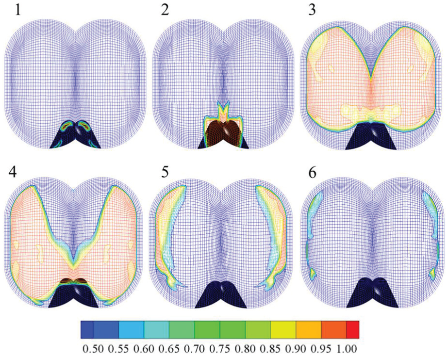
Figures 10–12 show the wet area of the inner surface of the buckets at the position of the same numbering as Figure 9. Despite different rotational speeds, the patterns of the wet area in each case have some common features. From the viewpoint of a bucket, the impingement starts at the cut-out with the water jet coming diagonally from the bottom so that the water is spreading to the upper part of the bucket. The impinging point of the water jet is moving to the center of the bucket and the corresponding incidence angle of the jet is also increasing. When the bucket is vertical to the jet, water sheet is coming out from the center point and is pushed out in the horizontal direction. After the bucket passes over the design point, the impinging point moves back to the cut-out and the water jet comes diagonally from the top, consequently the water sheet going out through the bottom part of the bucket. This repeated process is also observed in the numerical results of other researches.^1,6,7

Figure 10.

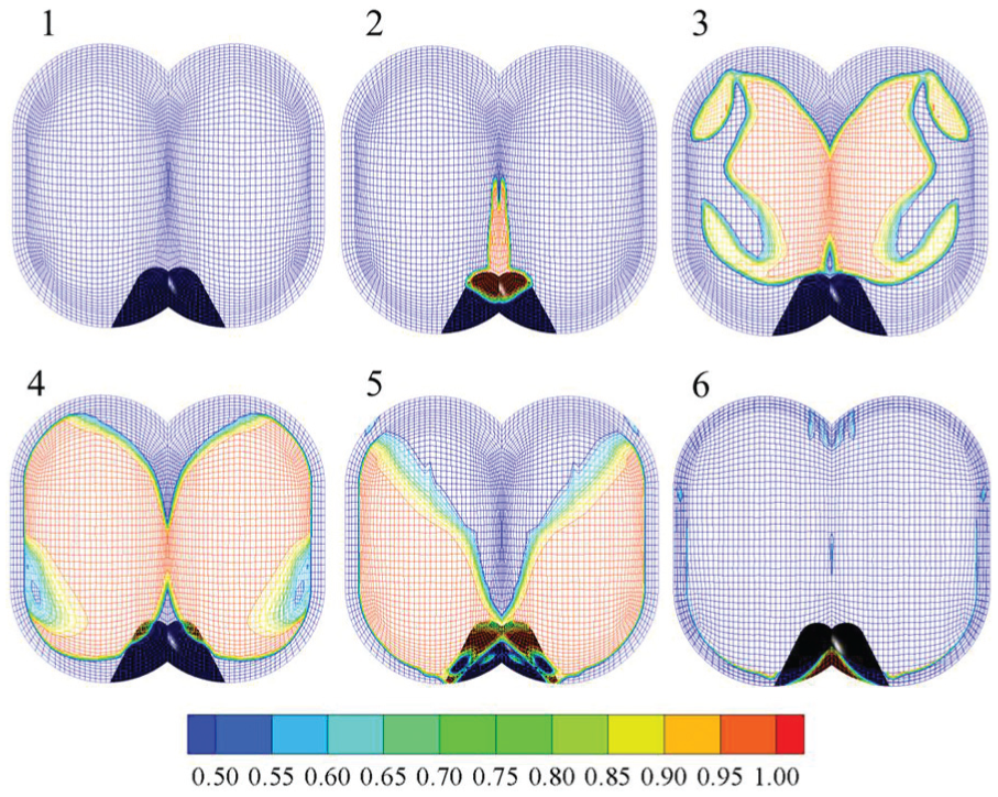
Water volume fraction on bucket inner surface at 800 r/min.

Figure 11.

Water volume fraction on bucket inner surface at 600 r/min.

Figure 12.

Water volume fraction on bucket inner surface at 400 r/min.

However, different rotational speeds of the turbine runner cause some differences in the wet area of the bucket. At 800 r/min, in Figure 10, the impingement of the water jet starts on bucket 2 and finishes on bucket 5. Before the impact of the other jet from the lower injector, the inner surface of bucket 6 is completely empty of water. At 600 r/min, in Figure 11, the water jet impingement lasts till bucket 5, but water sheet still exists in both sides on bucket 6. At 400 r/min, in Figure 12, the water jet impingement finishes on bucket 4, and the water sheet moves to the side in the horizontal direction thereafter. As the rotational speed of the turbine runner increases, the impinging time per revolution of a bucket also increases, but the effective impinging time becomes short. At a lower rotational speed, the effective impinging time occupies most of the impinging time although it is short. Therefore, the optimum operating speed of the turbine runner can be determined by the trade-off between the impinging time and the effective impinging time.

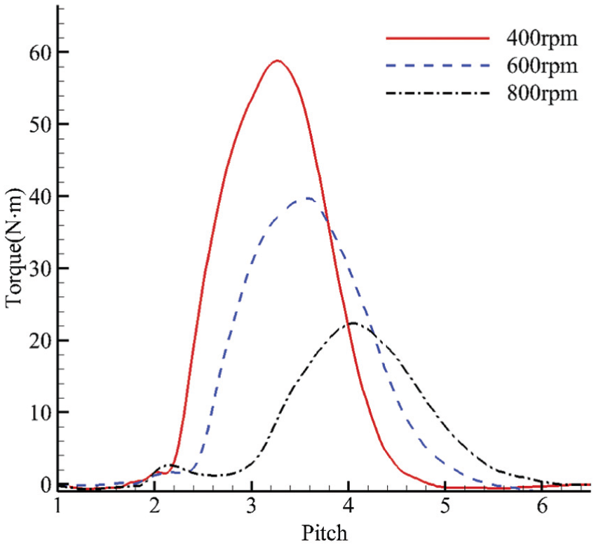
Figure 13 shows torque variation of a bucket during the water jet impingement from the upper nozzle. The starting position of a bucket was set to be the same in all speeds. The water jet started impinging on the cut-out of the bucket around 1.8 pitch position, and the torque increases slightly in all cases. However, the torque variation after the initial impingement shows totally different behaviors depending on the turbine runner speed. It is evident that the maximum value of torque decreases and the moment with the maximum torque is delayed from the starting point, as the runner speed increases. The bucket has the maximum torque around 3, 3.5, and 4 pitch positions for 400, 600, and 800 r/min, respectively. The position of the bucket with the maximum torque corresponds to the position of the bucket completely filled with water sheet as shown in Figures 10–12. The position of the maximum torque at only 600 r/min matches the position of a bucket vertical to the jet in Figure 9, and the turbine has the maximum efficiency at this speed. Another important thing is the duration of the impingement. The torque of a bucket has a positive value when the water jet hits the inner surface of the bucket. Therefore, the duration of the impingement per revolution increases as the bucket speed increases. It is evident that the influence of the upper nozzle on the bottom nozzle is marginal because the wet area in the inner surface of each bucket is very small, as shown in Figures 10–12, and the torque of each bucket goes to zero, as shown in Figure 13, just before each bucket is hit by the bottom nozzle.

Figure 13.

Torque variation of a bucket by water jet.

Applying Euler turbine equation to Pelton turbine suggested by Munson et al., ¹⁰ torque on the shaft can be derived as the following equation

$$\mathrm{\tau }=-\stackrel{·}{\mathrm{m}}\mathrm{R}(\mathrm{U}-{\mathrm{V}}_{\mathrm{j}})(1-\cos \mathrm{\beta })$$

(4)

The torque on the shaft is directly linear to the rotational speed in theory, but actual torque is not linear to the wheel speed as shown in Figure 14. In the derivation of equation (4), it is assumed that the jet always hits the bucket splitter in the vertical direction and leaves after turning of angle β. In the simulation results of the real Pelton turbine, the incidence angle of the jet is periodically changing depending on the position of a bucket relative to the jet, and the effective impinging time with the nearly vertical jet significantly decreases as the wheel speed increases. Therefore, the decrement of torque between two different rotational speeds increases considerably with the increase in the rotational speed.

Figure 14.

Time-averaged torque of Pelton turbine runner at different speeds.

Conclusions

Small Pelton turbine was numerically tested to analyze the performance and internal flow at five different wheel speeds. The following conclusions were drawn from a comparison of the numerical results:

1. A new grid topology of hexahedral meshes without any tetrahedral mesh was suggested to generate the computational mesh around the complex geometry of a bucket. The predicted flow coefficient, head coefficient, and overall efficiency agreed well with the experimental data.

2. Numerical diffusion of the water jet was observed across the interface between the runner and the casing domains. Extra caution is necessary to select the grid resolution of the runner domain with trade-off between the numerical diffusion and the increased calculation time.

3. For a revolution, the impingement of the water jet increases in time, but the portion of the effective impinging time decreases as the turbine runner rotates faster. At a slower speed of the wheel, the impinging time was short but effective to increase torque as theory with nearly vertical water jet.

4. The torque generated by a bucket is closely related to the water sheet on the inner surface of the bucket. Regardless of the rotating speed, the torque has a maximum value when the water sheet fills the inner surface completely.

5. The maximum efficiency of a Pelton turbine can be achieved with the optimum operating speed of a turbine runner, at which the maximum torque occurs when the water jet from the injector impinges a bucket in the vertical direction.