Real-time traffic signal optimization model based on average delay time per person

Abstract

Real-time traffic signal control is very important for relieving urban traffic congestion. Many existing traffic control models were formulated using optimization approach, with the objective functions of minimizing vehicle delay time. To improve people’s trip efficiency, this article aims to minimize delay time per person. Based on the time-varying traffic flow data at intersections, the article first fits curves of accumulative arrival and departure vehicles, as well as the corresponding functions. Moreover, this article transfers vehicle delay time to personal delay time using average passenger load of cars and buses, employs such time as the objective function, and proposes a signal timing optimization model for intersections to achieve real-time signal parameters, including cycle length and green time. This research further implements a case study based on practical data collected at an intersection in Beijing, China. The average delay time per person and queue length are employed as evaluation indices to show the performances of the model. The results show that the proposed methodology is capable of improving traffic efficiency and is very effective for real-world applications.

Introduction

In recent years, China is developing very fast in economy, urbanization, and motorization. Meanwhile, traffic problems caused by the sharp growth of vehicle ownership and traffic flows have already become serious obstacles to urban development. Advanced traffic management system (ATMS) is one of the important approaches to improve the traffic operation efficiency and also a key symbol of the modernization of the city. As the main method of urban traffic management, traffic signal control plays a significant role in the ATMS.

Many researches have focused on optimization of traffic signal timing. As the pioneering work, Miller ¹ proposed a fixed time signal control model to achieve the minimum average delay time. Along the same direction, Gazis ² and D’Ans and Gazis ³ also employed minimum delay time as objective function and formulated some traffic signal optimization models. Besides delay time, Michalopoulos and Stephanopoulos^4–6 further integrated the queue length constraints into the optimization and considered the spillback phenomenon. Using rather similar method, Akcelik ⁷ presented an objective function considering both number of stops and delay time, which was called ARRB (Australian Road Research Board) method. Based on interrelations between signal parameters (cycle length, split, etc.) and evaluation indices (delay time, queue length, number of stops, etc.), all the above models were formulated using mathematical programming methods.

Recently, some researches have combined some evaluation indices together and formulated some multi-objective traffic control models to seek simultaneous optimization of several objectives. Lieberman et al. ⁸ presented a real-time model for arterials incorporating three objectives, including maximum system throughput, maximum usage of storage capacity, and equitable service. Ceder and Reshetnik ⁹ proposed two signal models for under-saturated and over-saturated intersections, respectively, using minimization of maximum queue length and accumulative queue length as two objective functions. Furthermore, Talmor and Mahalel ¹⁰ integrated the maximum capacity into objectives of traffic signal control to improve the intersection capacity. Schmocker et al. ¹¹ formulated a multi-objective optimization model based on three evaluation indices, mean delay of vehicles at the intersection, mean queue length and the waiting time of pedestrians crossing the intersection, and incorporated a fuzzy logic in the model. Li ¹² established a multi-objective optimization model for large traffic and pedestrian flows. Jiao and Sun ¹³ proposed a multi-objective optimization model to minimize delay time and queue length and to maximize effective capacity simultaneously and applied the methodology to a practical intersection in Beijing, China. All the above multi-objective models were also represented using mathematical programming approaches.

Besides the above-mentioned mathematical optimization models, some simulation-based approaches have also been developed. A rather famous one in early years is Traffic Network Study Tool (TRANSYT) explained by Robertson, ¹⁴ Wallace et al., ¹⁵ and Wong. ¹⁶ Some real-time traffic control systems were further developed based on time-varying traffic flows, such as Split, Cycle and Offset Optimization Technique (SCOOT),^17,18 Sydney Coordinated Adaptive Traffic System (SCATS),^19,20 Real-time Hierarchical Optimized Distributed and Effective System (RHODES), ²¹ and Optimized Policies for Adaptive Control (OPAC). ²² All the above simulation-based systems have been applied in real-world traffic signal control and solved many traffic problems. However, due to more complicated traffic conditions, especially the mixed traffic flow, these systems are not appropriate for Chinese situations.

In both mathematical programming approaches and simulation-based systems, minimum delay time at intersection is a very important objective. However, almost all the existing researches only pay attention to the delay time of vehicles, because car is the most predominant on the road in the western countries. In China, public transportation is a kind of very important trip mode, which carries much more people than car and is much more efficient. Additionally, most Chinese cities are facing very serious mixed traffic flow conditions; conflicts among pedestrian, cyclist, and vehicle are rather severe, ²³ and drivers’ characteristics of various vehicle types are greatly different. ²⁴ Therefore, in Chinese situation, the delay time per person should be more important.

The key point of this article is to transfer delay time per vehicle to delay time per person and employ it as the objective to formulate a real-time traffic control model. The article is organized in five sections. Following the introduction in the first section, the delay time of vehicle at intersections is discussed in the second section, as well as the delay time per person. The real-time traffic control model is formulated in the third section. The case study results are reported in the fourth section to demonstrate the performances of the proposed model. Conclusions and further research directions are summarized in the last section.

Delay time at intersections

Basic interpretation

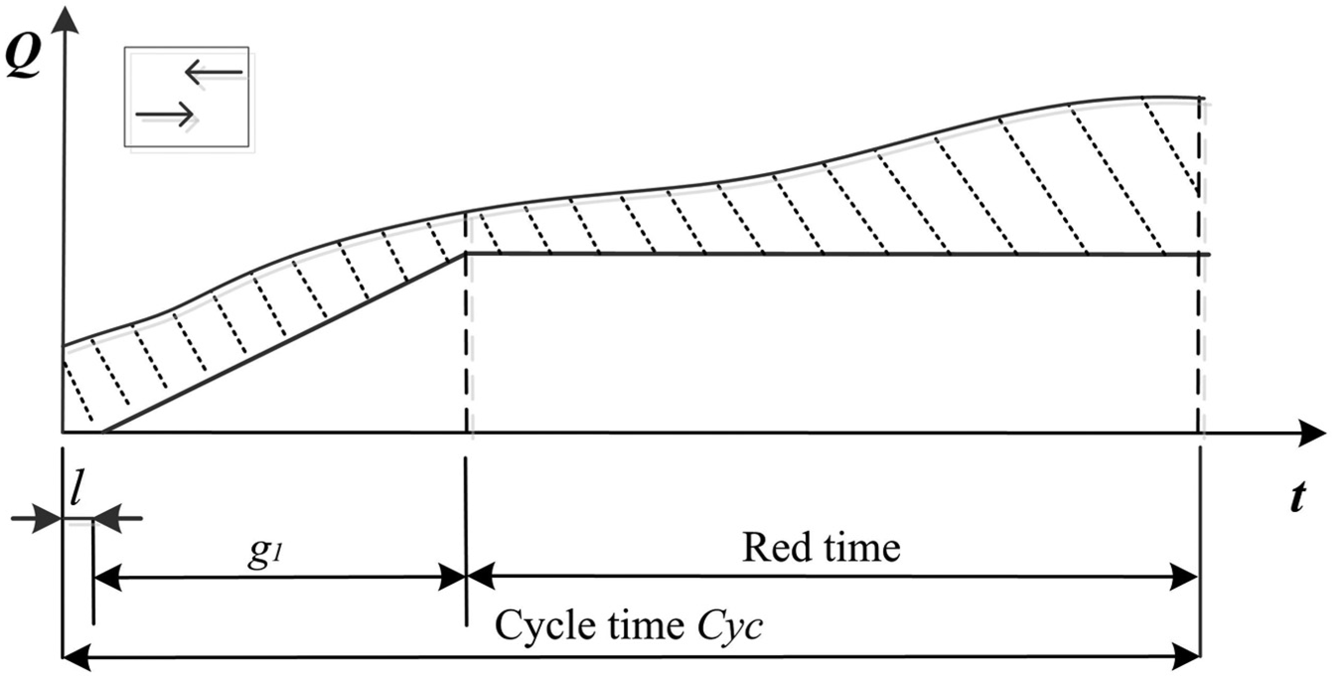
The arrival and departure processes of vehicles at the entrance legs at intersections are illustrated in Figure 1.

Figure 1.

Arrival and departure of vehicles.

In the above figure, the variables are defined as follows:

• t: horizontal axis, denoting the time;

• Q: vertical axis, showing the number of accumulative vehicles;

• x: start time of red phase;

• r: length of red phase;

• g_b : dispersion time of queuing vehicles;

• g: green time;

• Cyc: cycle length;

• f(t): function of accumulative arrival vehicles, that is, the curve ABH;

• $\phi (t)$ : function of accumulative departure vehicles, that is, the curve CBH;

• Q ₀: stranded vehicles during the last cycle.

During the green phase time g, some vehicles will arrive after the queue dispersion finishes, and these vehicles will pass through the intersection without delay.

Using D_z to denote the total delay time during one cycle, which equals to the area of ABCD, that is

$$D_z=S_{\text{DABF}}-S_{\text{CBF}}=\underset{x}{\overset{x+r+g_b}{\int }}f(t)\mathrm{dt}-\underset{x+r}{\overset{x+r+g_b}{\int }}\phi (t)\mathrm{dt}$$

(1)

where $S_{\text{DABF}}$ denotes the area of DABF, and $S_{\text{CBF}}$ shows the area of CBF.

Delay time of vehicles

For a typical four-phase intersection in this article, the curves of accumulative arrival and departure vehicles during each phase are expressed in Figures 2–5, respectively. The upper curve denotes arrival vehicles, while the lower one shows departure vehicles. Here, sequence of phases is defined as follows: (1) go straight at east and west legs, (2) left-turn at east and west legs, (3) go straight at north and south legs, and (4) left-turn at north and south legs. In this article, the right-turn direction is allowed during all signal phases.

Figure 2.

Arrival and departure vehicles: go straight at east and west legs

Figure 3.

Arrival and departure vehicles: left-turn at east and west legs.

Figure 4.

Arrival and departure vehicles: go straight at north and south legs.

Figure 5.

Arrival and departure vehicles: left-turn at north and south legs.

Some symbols are further defined as follows:

• i: entrance legs, where E is the east entrance, W is the west entrance, N is the north entrance, and S is the south entrance;

• j: heading direction, that is, $j=1$ means go straight, and $j=2$ means left-turn;

• k: vehicle type, that is, $k=1$ means bus, and $k=2$ means car;

• l: loss time between two consecutive phases;

• d_ijk : delay time of vehicle type k entering from entrance leg i heading to direction j;

• t_ijk : dispersion time of vehicle type k entering from entrance leg i heading to direction j;

• $f_{\mathrm{ijk}}(t)$ : function of accumulative arrival vehicle type k entering from entrance leg i heading to direction j;

• ${\phi }_{\mathrm{ijk}}(t)$ : function of accumulative departure vehicle type k entering from entrance leg i heading to direction j;

• g_p : effective green time during phase p, $p=1,2,3,4$ .

For vehicles going straight at east and west entrance legs, the combinations of i, j, and k include E11, E12, W11, and W12, that is, bus going straight from the east leg, car going straight from the east leg, bus going straight from the west leg, and car going straight from the west leg.

From Figure 2, we formulate the delay time during phase 1 as the following equation

$$\begin{array}{c}\multicolumn{1}{c}{d_{\mathrm{ijk}}=\underset{0}{\overset{l+g_1}{\int }}{f}_{\mathrm{ijk}}(t)\mathrm{dt}-\underset{0}{\overset{l+g_1}{\int }}{\phi }_{\mathrm{ijk}}(t)\mathrm{dt}}\\ \multicolumn{1}{c}{+\underset{l+g_1}{\overset{\mathrm{Cyc}}{\int }}{f}_{\mathrm{ijk}}(t)\mathrm{dt}-\underset{l+g_1}{\overset{\mathrm{Cyc}}{\int }}{\phi }_{\mathrm{ijk}}(t)\mathrm{dt}}\end{array}$$

(2)

Actually, the result from equation (2) shows the area of the shadow. For vehicles turning left at east and west entrance legs, the combinations of i, j, and k include E21, E22, W21, and W22, that is, bus turning left from the east leg, car turning left from the east leg, bus turning left from the west leg, and car turning left from the west leg.

From Figure 3, we formulate the delay time during phase 2 as the following equation

$$d_{\mathrm{ijk}}=\underset{0}{\overset{\mathrm{Cyc}}{\int }}{f}_{\mathrm{ijk}}(t)\mathrm{dt}-\underset{r+l}{\overset{r+l+g_2}{\int }}{\phi }_{\mathrm{ijk}}(t)\mathrm{dt}-\underset{r+l+g_2}{\overset{\mathrm{Cyc}}{\int }}{\phi }_{\mathrm{ijk}}(t)\mathrm{dt}$$

(3)

where

$$r_2=l+g_1$$

(4)

For vehicles going straight at north and south entrance legs, the combinations of i, j, and k include N11, N12, S11, and S12, that is, bus going straight from the north leg, car going straight from the north leg, bus going straight from the south leg, and car going straight from the south leg.

From Figure 4, we formulate the delay time during phase 3 as the following equation

$$d_{\mathrm{ijk}}=\underset{0}{\overset{\mathrm{Cyc}}{\int }}{f}_{\mathrm{ijk}}(t)\mathrm{dt}-\underset{r_3+l}{\overset{r_3+l+g_3}{\int }}{\phi }_{\mathrm{ijk}}(t)\mathrm{dt}-\underset{r_3+l+g_3}{\overset{\mathrm{Cyc}}{\int }}{\phi }_{\mathrm{ijk}}(t)\mathrm{dt}$$

(5)

where

$$r_3=2l+g_1+g_2$$

(6)

For vehicles turning left at north and south entrance legs, the combinations of i, j, and k include N21, N22, S21, and S22, that is, bus turning left from the north leg, car turning left from the north leg, bus turning left from the south leg, and car turning left from the south leg.

From Figure 5, we formulate the delay time during phase 4 as the following equation

$$d_{\mathrm{ijk}}=\underset{0}{\overset{\mathrm{Cyc}}{\int }}{f}_{\mathrm{ijk}}(t)\mathrm{dt}-\underset{r_4+l+g_4}{\overset{\mathrm{Cyc}}{\int }}{\phi }_{\mathrm{ijk}}(t)\mathrm{dt}$$

(7)

where

$$r_3=3l+g_1+g_2+g_3$$

(8)

Equations (2), (3), (5), and (7) show vehicle delay time during four phases, respectively.

Delay time per person

The purpose of this research is to minimize the average delay time per person. Here, both drivers and passengers in the bus and car are included. For convenience, we divide 1 h into N intervals. Some variables are defined as follows:

• ${\beta }_{\mathrm{ijn}}$ : average passenger load of bus entering from leg i heading to direction j during interval n, $n=1,2,\dots ,N$

• ${\alpha }_{\mathrm{ijn}}$ : average passenger load of car entering from leg i heading to direction j during interval n, $n=1,2,\dots ,N$

• $x_{\mathrm{ijn}}$ : number of buses entering from leg i heading to direction j during interval n, $n=1,2,\dots ,N$

• $y_{\mathrm{ijn}}$ : number of cars entering from leg i heading to direction j during interval n, $n=1,2,\dots ,N$

The total delay time of all vehicles during one cycle is then formulated as

$$D\prime =\sum _i\sum _j\sum _k{d}_{\mathrm{ijk}}$$

(9)

Using $D$ to indicate the average delay time per person during 1 h, then

$$D=\frac{D\prime }{\sum _{\mathrm{ijn}}({\beta }_{\mathrm{ijn}}{x}_{\mathrm{ijn}}+{\alpha }_{\mathrm{ijn}}{y}_{\mathrm{ijn}})}·\frac{3600}{\mathrm{Cyc}}$$

(10)

Equation (10) shows the average delay time per person at intersections, which is also employed as the objective function in this research.

Real-time traffic control model based on delay time per person

For a typical four-phase intersection, we further define the following symbols:

• L: total loss time during one cycle

• g _min: minimum green time

• g _max: maximum green time

• $\mathrm{Cy}{c}_{min}$ : minimum cycle length

• $\mathrm{Cy}{c}_{max}$ : maximum cycle length

Based on equations (2), (3), (5), (7), (9), and (10), the real-time traffic control model based on delay time per person is then formulated as

$$\begin{array}{c}\multicolumn{1}{c}{minD(g_p)=\frac{\sum _i\sum _j\sum _k{d}_{\mathrm{ijk}}}{\sum _{\mathrm{ijn}}({\beta }_{\mathrm{ijn}}{x}_{\mathrm{ijn}}+{\alpha }_{\mathrm{ijn}}{y}_{\mathrm{ijn}})}·\frac{3600}{\mathrm{Cyc}}}\\ \multicolumn{1}{c}{s.t.\{\begin{array}{c}\hfill \sum _{p=1}^4{g}_p+L=\mathrm{Cyc}\hfill \\ \multicolumn{1}{c}{\mathrm{Cy}{c}_{min}\le \mathrm{Cyc}\le \mathrm{Cy}{c}_{max}}\\ \multicolumn{1}{c}{g_{min}\le g_p\le g_{max}}\end{array}}\end{array}$$

(11)

In this article, the average passenger loads of bus and car are obtained through field survey. Moreover, the loss time during one cycle is taken as 16 s, the minimum green time is taken as 5 s, the maximum green time is taken as 45 s, the minimum cycle length is 36 s ( $\mathrm{Cy}{c}_{min}=5\times 4+16=36$ ), and the maximum cycle length is 196 s ( $\mathrm{Cy}{c}_{max}=45\times 4+16=196$ ).

Since there exist some integrals in the real-time traffic control model, it is difficult to be solved using traditional optimization algorithms. In this article, we code the model using M language based on the MATLAB platform.

Case study

To testify performances of the proposed real-time traffic control model, we implemented a field survey in a weekday morning at the intersection of Garden Bridge in Beijing, China. We collected real-world time-varying data of 3 h from 7 a.m. to 10 a.m., including traffic volume (all vehicle types), average passenger load, existing signal timing parameters, and geometric features of the intersection. We also collected the existing delay time and queue length for evaluation. Specially, we record the exact arrival and departure time of each vehicle and then obtained the curves of both accumulative arrival and departure vehicles. The passenger loads of all buses and cars were also collected to transfer vehicle delay time to average delay per person. All the above field data provided rather rich information for both input and evaluation indices in the case study. The lane composition of the case intersection is described in Figure 6.

Figure 6.

Intersection layout.

The existing signal timing is shown in Figure 7. The cycle length is 193 s, with all yellow time and all red time as 3 s.

Figure 7.

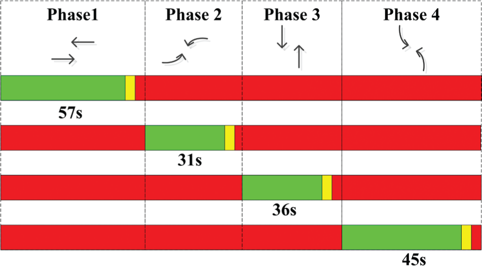
Existing signal timing.

Model solution

In this research, we use polynomial function to show the characteristics of accumulative arrival and departure vehicles, that is

$$y=a{t}^2+\mathrm{bt}+c$$

(12)

where y is the number of accumulative vehicles, t is the time index from the starting point, and a, b, and c are the parameters to be estimated. Based on the exact arrival and departure time of each vehicle from the survey, we first get estimations of a, b, and c using least square approach, and then we obtain the detailed formulation of $f_{\mathrm{ijk}}(t)$ and ${\phi }_{\mathrm{ijk}}(t)$ , as well as the corresponding curves. Moreover, we input these curves and corresponding polynomial functions into our MATLAB code and obtain optimized signal cycle and green time.

A very important issue in the solution process is that we employ a rolling horizon method to realize the real-time signal control, that is, once we obtain the optimized signal parameters (including cycle length and green time) during one cycle, we update the functions of accumulative arrival and departure vehicles according to the new signal timing, and the signal parameters during the next cycle will keep updating with this process.

Optimized real-time signal parameters are reported in Table 1 and Figure 8. Here, phase 1 means go straight at east and west legs, phase 2 shows left-turn at east and west legs, phase 3 indicates go straight at north and south legs, and phase 4 is left-turn at north and south legs. Yellow time is 3 s, and all red time is 1 s.

Table 1.

Real-time signal parameters (unit: s).

No.	Phase 1	Phase 2	Phase 3	Phase 4	Cycle	No.	Phase 1	Phase 2	Phase 3	Phase 4	Cycle
1	34	30	33	24	137	33	42	45	42	41	186
2	34	30	33	31	144	34	45	45	42	41	189
3	35	31	33	26	141	35	42	45	42	43	188
4	34	32	32	25	139	36	44	45	40	39	184
5	34	30	28	24	132	37	45	45	43	41	190
6	36	35	33	31	151	38	44	43	42	40	185
7	34	30	33	26	139	39	42	45	42	40	185
8	34	30	35	30	145	40	43	45	41	38	183
9	33	35	33	29	146	41	44	44	43	40	187
10	34	32	32	25	139	42	45	45	43	40	189
11	34	30	33	26	139	43	45	44	41	39	185
12	36	29	33	30	144	44	43	45	44	40	188
13	34	30	33	26	139	45	45	45	42	38	186
14	37	38	30	29	150	46	44	43	41	36	180
15	40	39	39	30	164	47	44	43	40	40	183
16	39	41	40	36	172	48	43	42	41	34	176
17	34	30	39	32	151	49	43	44	39	35	177
18	36	29	41	38	160	50	42	41	40	32	171
19	39	41	39	34	169	51	43	40	41	33	173
20	41	44	43	35	179	52	40	39	39	34	168
21	38	45	40	38	177	53	42	38	39	33	168
22	38	45	39	38	176	54	40	39	33	31	159
23	42	43	42	34	177	55	41	42	41	33	173
24	42	45	44	33	180	56	38	30	33	26	143
25	45	45	44	40	190	57	38	30	33	26	143
26	44	45	40	35	180	58	36	29	32	25	138
27	43	45	38	32	174	59	32	30	33	26	137
28	45	45	43	39	188	60	39	35	34	32	156
29	45	45	44	40	190	61	33	30	31	26	136
30	45	45	42	38	186	62	34	29	31	26	136
31	44	45	43	39	187	63	34	30	33	26	139
32	44	45	43	39	187	64	34	32	32	25	139
						65	34	28	33	26	137

Figure 8.

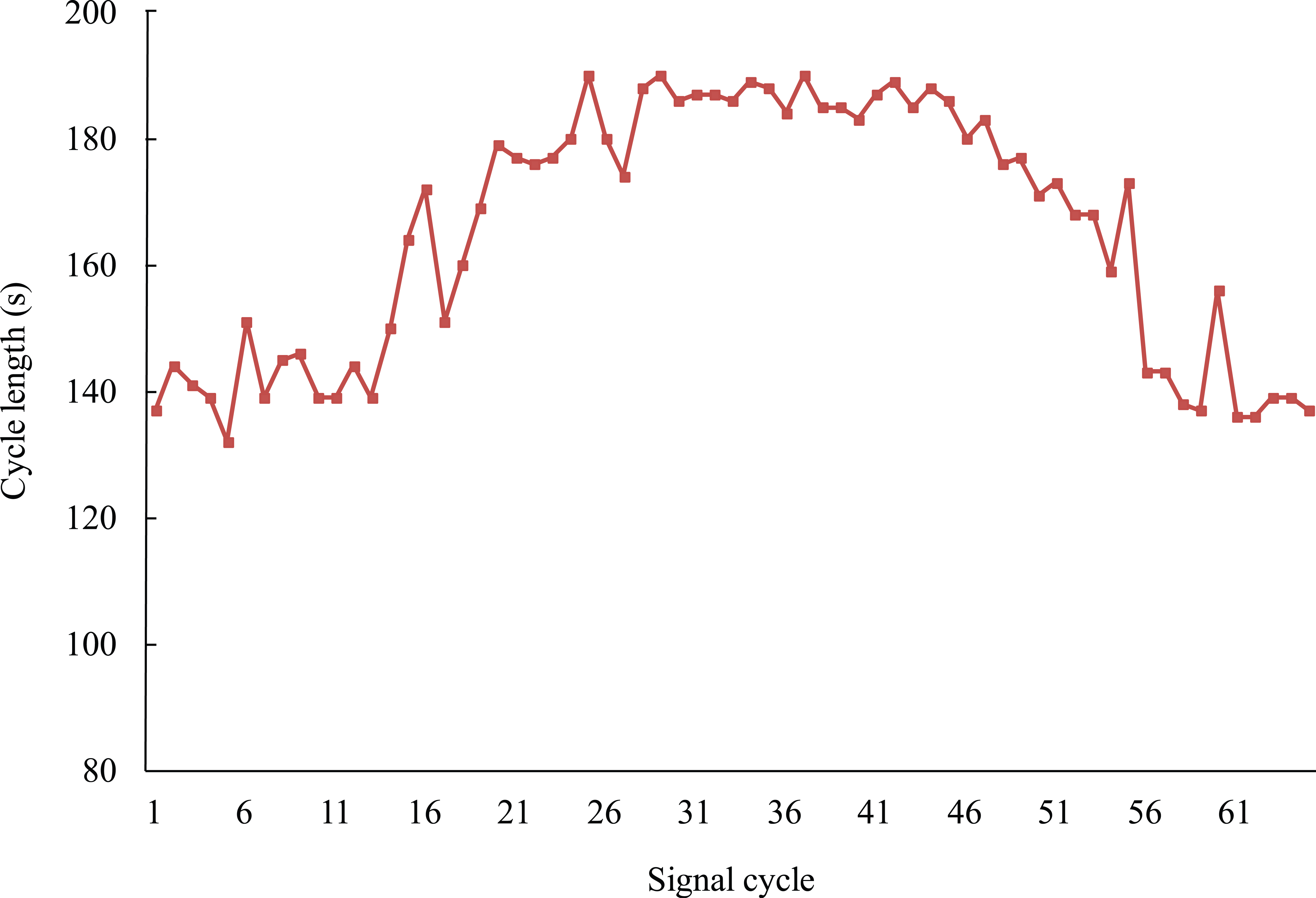
Real-time signal cycle from the proposed model.

From the time-varying 65 signal cycles in 3 h, we can find out that the signal parameters update along with the trend of traffic flow, that is, the traffic control scheme is real-time in nature.

Model evaluation

Since it is impossible to adjust the signal plan in real world just for the purpose of this case study, we evaluate performances of the proposed model using traffic simulation technique. Here, we employed the software Vissim ²⁵ to simulate the proposed model.

The average delay time per person and average queue length are exported from the simulation for evaluation. Here, all evaluation indices are during the morning peak hour, that is, from 8 a.m. to 9 a.m.

Comparisons of delay time per person between the current scheme and optimized signal plan are summarized in Table 2, where the evaluation results of each 10 min are extracted to show detailed information. Graphical illustration is further shown in Figure 9.

Table 2.

Comparison of average delay time per person.

		8:00–8:10	8:10–8:20	8:20–8:30	8:30–8:40	8:40–8:50	8:50–9:00	Mean
E-S	Current (s)	75	36	65	26	54	35	48
	Proposed (s)	83	42	56	55	48	38	53
	Improvement (%)	−10.7	−16.7	13.8	−111.5	11.1	−8.6	−10.4
W-S	Current (s)	38	44	40	51	45	49	44
	Proposed (s)	40	41	50	42	46	51	45
	Improvement (%)	−5.3	6.8	−25.0	17.6	−2.2	−4.1	−2.3
E-L	Current (s)	88	80	45	34	67	42	59
	Proposed (s)	66	38	37	62	46	38	48
	Improvement (%)	25.0	52.5	17.8	−82.4	31.3	9.5	18.6
W-L	Current (s)	121	165	157	160	171	173	158
	Proposed (s)	34	41	42	44	41	43	41
	Improvement (%)	71.9	75.2	73.2	72.5	76.0	75.1	74.1
N-S	Current (s)	22	27	54	29	29	53	36
	Proposed (s)	19	42	37	32	64	21	36
	Improvement (%)	13.6	−55.6	31.5	−10.3	−120.7	60.4	0.0
S-S	Current (s)	47	36	43	30	41	38	39
	Proposed (s)	45	37	48	15	25	23	32
	Improvement (%)	4.3	−2.8	−11.6	50.0	39.0	39.5	17.9
N-L	Current (s)	38	62	112	108	104	104	88
	Proposed (s)	24	25	47	81	49	50	46
	Improvement (%)	36.8	59.7	58.0	25.0	52.9	51.9	47.7
S-L	Current (s)	126	112	108	103	113	135	116
	Proposed (s)	15	42	56	37	33	28	35
	Improvement (%)	88.1	62.5	48.1	64.1	70.8	79.3	69.8

E-S: go straight at east leg; W-S: go straight at west leg; E-L: left-turn at east leg; W-L: left-turn at west leg; N-S: go straight at north leg; S-S: go straight at south leg; N-L: left-turn at north leg; S-L: left-turn at south leg.

Figure 9.

Comparison of average delay time per person at all directions.

From Table 2 and Figure 9, we have the following results:

1. For all the turning directions at all entrance legs, the proposed model generates less delay time than the current scheme, that is, it outperforms the existing traffic signal timing.

2. The proposed model yields the best result for left-turn at west entrance leg, and the next one is left-turn at south entrance leg. According to traffic survey, left-turn faces rather severe traffic conflicts, and reasonable traffic control scheme could improve its efficiency greatly.

3. For go straight at east entrance leg, the proposed model gets a little worse result than the current scheme; however, it does not influence the general outstanding performances of the proposed model.

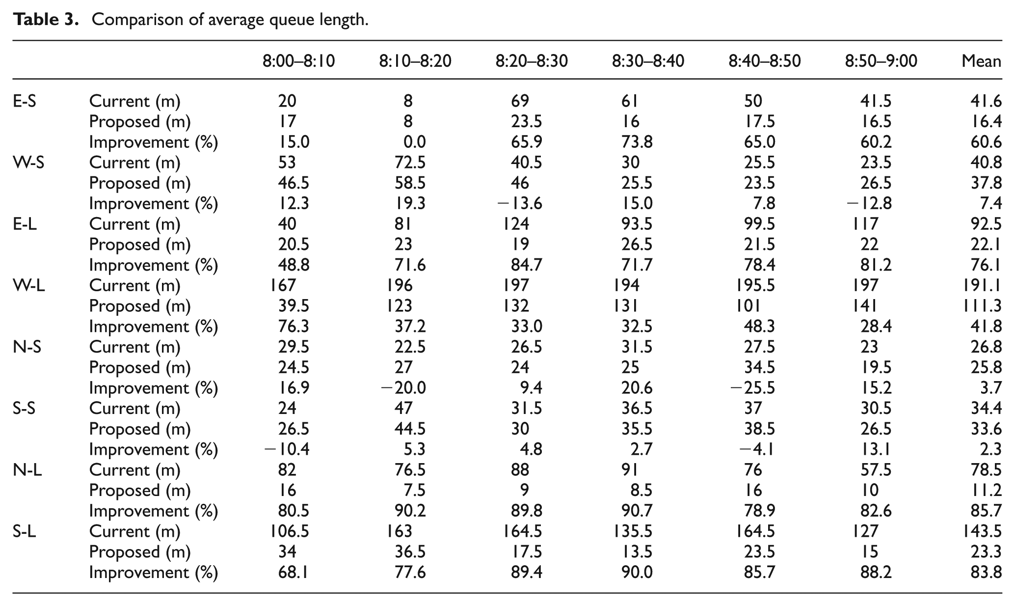
Similarly, comparisons of the average queue length between the current scheme and optimized signal plan are summarized in Table 3. Graphical illustration is further shown in Figure 10.

Table 3.

Comparison of average queue length.

		8:00–8:10	8:10–8:20	8:20–8:30	8:30–8:40	8:40–8:50	8:50–9:00	Mean
E-S	Current (m)	20	8	69	61	50	41.5	41.6
	Proposed (m)	17	8	23.5	16	17.5	16.5	16.4
	Improvement (%)	15.0	0.0	65.9	73.8	65.0	60.2	60.6
W-S	Current (m)	53	72.5	40.5	30	25.5	23.5	40.8
	Proposed (m)	46.5	58.5	46	25.5	23.5	26.5	37.8
	Improvement (%)	12.3	19.3	−13.6	15.0	7.8	−12.8	7.4
E-L	Current (m)	40	81	124	93.5	99.5	117	92.5
	Proposed (m)	20.5	23	19	26.5	21.5	22	22.1
	Improvement (%)	48.8	71.6	84.7	71.7	78.4	81.2	76.1
W-L	Current (m)	167	196	197	194	195.5	197	191.1
	Proposed (m)	39.5	123	132	131	101	141	111.3
	Improvement (%)	76.3	37.2	33.0	32.5	48.3	28.4	41.8
N-S	Current (m)	29.5	22.5	26.5	31.5	27.5	23	26.8
	Proposed (m)	24.5	27	24	25	34.5	19.5	25.8
	Improvement (%)	16.9	−20.0	9.4	20.6	−25.5	15.2	3.7
S-S	Current (m)	24	47	31.5	36.5	37	30.5	34.4
	Proposed (m)	26.5	44.5	30	35.5	38.5	26.5	33.6
	Improvement (%)	−10.4	5.3	4.8	2.7	−4.1	13.1	2.3
N-L	Current (m)	82	76.5	88	91	76	57.5	78.5
	Proposed (m)	16	7.5	9	8.5	16	10	11.2
	Improvement (%)	80.5	90.2	89.8	90.7	78.9	82.6	85.7
S-L	Current (m)	106.5	163	164.5	135.5	164.5	127	143.5
	Proposed (m)	34	36.5	17.5	13.5	23.5	15	23.3
	Improvement (%)	68.1	77.6	89.4	90.0	85.7	88.2	83.8

Figure 10.

Comparison of average queue length at all directions.

Once again, from Table 3 and Figure 10, we find out that the proposed model yields much shorter queue length than the existing scheme for all the turning directions at all entrance legs, and the best result appears at left-turn direction at north entrance leg. Generally, from the above evaluations, we can obtain the result that real-time traffic signal timing plans from the proposed model outperform existing scheme and are capable of improving efficiency of traffic management. It will lead to public transportation priority by minimizing average delay time per person.

Conclusion

This article presents a revised real-time traffic control model for intersections employing optimization approach. Different from the existing methods, the proposed model aims to minimize average delay time per person instead of delay of vehicles. We first fit curves of accumulative arrival and departure vehicles and formulate vehicle delay functions during each signal phase. Then we transfer vehicle delay time to personal delay time utilizing the average passenger load of cars and buses. Taking into account the necessary constraints, we further put forward the real-time traffic signal control model with the minimum delay time per person as the objective function. Field survey data at an intersection in Beijing are collected for case study. The reported results based on the practical data and simulation experiments show that signal timing from the proposed model keeps updating during each cycle and improves delay time per person and queue length at intersections greatly, especially at left-turn directions. Generally, the proposed model has rather outstanding performances, is very efficient for on-line applications in ATMS, and will lead to public transportation priority.

Future researches may consist of the following directions. The first is to further take into account cyclists and pedestrians and to formulate a real-time signal control model under mixed traffic flow conditions. The second is to integrate upstream and downstream intersections to present an arterial coordination control model. The third is to combine some other objectives together and to put forward some multi-objective traffic signal optimization models.