Study on the application of dimensionality reduction method on reliability and reliability sensitivity analysis of random vibration systems

Abstract

The application of dimensionality reduction method on the reliability and reliability sensitivity analysis of vibration systems was examined. The dimensionality of a vibration reliability problem was reduced to only two independent dimensions by the means of polar transformation. As the safe and failure classes of samples are clearly distinguishable and occupy a standard position in a two-dimensional plot in the case that the important direction exists, the relevant samples are selected visually. The reliability and reliability sensitivity problems were solved using the position of the relevant samples. Before the reliability and reliability sensitivity estimation, an essential visualization analysis is conducted to examine the capacity of the method in terms of the existence of the important direction which is used to reduce the dimensionality of the reliability problem. In order to calculate the design point correctly, the improved Hasofer–Lind–Rackwitz–Fiessler method was extended with a procedure for determining the perturbation in the calculation of the gradient vector by finite differences according to the numerical precision of the limit state function. The dimensionality reduction method saves the numbers of calling limit state function a lot and has the same accuracy as Monte Carlo method. Examples involving single and multiple degree-of-freedom nonlinear vibration systems were used to demonstrate the approach.

Introduction

The treatment of systems with uncertain structural parameters has become an increasingly important issue in many areas of dynamic analysis. The parameter uncertainties in dynamic systems are due to material irregularity, manufacturing tolerance, and measurement inaccuracies, which are usually modeled as random variables or stochastic process. The performance uncertainties of the systems such as displacements, stress state, and vibration frequencies should be studied effectively for design purpose. Because that the dynamic response of a mechanical system with uncertain parameters possesses probabilistic features which depend on the probabilistic distribution of the system parameters, the study of the stochastic responses of structures with uncertain parameters is of significant interest in many engineering applications. In recent years, a series of papers^1–6 have shown that the failure problem of vibration systems can be solved by applying the computational tools of structural reliability methods. In these approaches, the failure event of a vibration system is expressed as implicit functions of the input uncertainties, that is, the limit state functions of the system. Structural reliability methods are then used to calculate the reliability of the vibration system. Reliability sensitivity analysis has been widely applied in reliability engineering design to estimate the effect of change in random variables on the probability of failure. It can help designer to establish acceptable parameter values on the structures and to select acceptable tolerances and parameters.^7–9 In order to assess the effects of the uncertain parameters on the reliability of the vibration systems and to determine the main factors influencing the systems reliability, structural reliability sensitivity analysis methods have been widely applied.^10–13 A source of difficulties for solving the vibration reliability and reliability sensitivity problems by means of approximate methods, for example, first-order reliability method (FORM) and second-order reliability method (SORM), is the structural nonlinearity. It is due to the fact that the surrogate of the limit state functions built by approximate methods may be inaccurate when the systems have strong nonlinearities. Despite Monte Carlo method (MCM) is the most general simulation technique, a large number of calling the limit state function is required in estimating probabilities of rare occurrence events and the numerical cost may be high, especially when the system is modeled using nonlinear differential equations. Different advanced simulation techniques have been developed to overcome the inefficiency of MCM, but the robustness of the methods remains to be improved. JE Hurtado ¹⁴ introduced the dimensionality reduction method (DRM) and applied it to structural reliability problems successfully. In this approach, the samples in the standard normal space are mapped to a two-dimensional (2D) plot defined by the polar features of the samples, that is, the length of the sample vector and the cosine of the angle that separates the sample vector and the important direction. Due to the fact that the safe and failure classes of samples are clearly distinguishable and occupy a standard position in the plot, the reliability problem is solved by a visually aided selection of the relevant samples. The method facilities the numerical computation of the reliability and has the same accuracy as MCM. However, it needs to be examined when applied to vibration reliability problems. A surrogate of the important direction is given by the design point vector, which can be determined by the well-known improved Hasofer–Lind–Rackwitz–Fiessler (iHLRF) method^15,16 efficiently. When the limit state function is defined from a numerical model, for example, nonlinear differential equations, the gradient vector is computed approximately by finite difference, which may lead to errors if the perturbation is not correctly chosen. In the case that the shape of failure region is very involved, the existence of important direction is questionable. ¹⁷

In this study, the DRM is first applied to random vibration systems to reduce the dimensionality of the vibration reliability problem by transforming the excitation process into a finite set of standard normal random variables. Then, a visualization analysis is conducted to examine the clustering feature of the samples and the existence of important direction is extensively discussed by analyzing a Duffing oscillator. In order to reduce the number of times of calling the limit state function, the iHLRF method for finding the design point is extended with a procedure for determining the perturbation in the calculation of the gradient vector by finite difference according to the numerical precision of the limit state function. Based on these, an integrated strategy for reliability and reliability sensitivity estimation of random vibration system with random structural parameters is finally presented using the relevant samples in a 2D plot. Two numerical examples are used to demonstrate the accuracy and efficiency of the strategy and the effects of the structural random parameters on reliability of a multiple degree-of-freedom impacting system are finally studied.

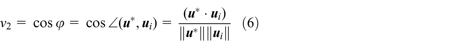
Dimensionality reduction of vibration reliability problems

Vibration reliability problems in the standard normal space

It is known that the differential equations of motion of a vibration system can be written as follows

$$\mathit{f}[\stackrel{··}{\mathit{r}}(t),\stackrel{·}{\mathit{r}}(t),\mathit{r}(t),\mathit{v}]=\mathit{F}(t)$$

(1)

where t denotes the time; f (·) is a vector of polynomial functions; r (t) is the response vector; v is a vector of system parameters that characterize the mass, damping, and stiffness; and F (t) is a vector of external excitation. In vibration reliability problems, our concern lies in estimating the probability that the response r(t) at a given time exceeds a specified threshold for prescribed probabilistic description of v and F (t). In order to solve the problem by structural reliability methods, each stochastic process F(t) is represented in the form of a finite number of random variables^1,5,6,18 as follows

$$F(t)=\sum _{i=1}^n{w}_i{s}_i(t)=\mathit{s}{(t)}^{\mathrm{T}}\mathit{w}$$

(2)

where w is a vector of n-dimensional independent normal variables and s (t) is a vector of n-dimensional deterministic functions of time. Thus, the vibration reliability problem is defined by the vectors of random variables v and w and the response vector is an implicit function of these random variables, that is, r = r ( v , w , t). When the failure event is defined as that the response r at a given time t ₀ exceeds a specified threshold b, the limit state function of the reliability problem is

$$g(\mathit{v},\mathit{w},t_0,b)=b-r(\mathit{v},\mathit{w},t_0)$$

(3)

the failure probability P _f = P{b < r( v , w , t ₀)} = P{g( v , w , t ₀, b) < 0)}.

Let u = ( u_v , u_w ) with u_v = T _v ( v ) and u_w = T _w ( w ), where T(·) is the Rosenblatt or Nataf transformation such that u is a vector of standard normal variables. Then, the limit state function (3) can be written as follows

$$g(\mathit{v},\mathit{w},t_0,b)=g[{\mathrm{T}}_{\mathit{v}}^{-1}({\mathit{u}}_{\mathit{v}}),{\mathrm{T}}_{\mathit{w}}^{-1}({\mathit{u}}_{\mathit{w}}),t_0,b]\equiv G(\mathit{u},t_0,b)$$

(4)

the failure probability P _f = P{G( u , t ₀, b) < 0}; thus, the vibration reliability problem is defined in the standard normal space.

Polar transformation

Consider a sample u _i = (u ₁, u ₂...u_d ) of a vibration reliability problem in the standard normal space, where d is the dimensionality of the space. The polar features are defined as the length l of the sample u _i and the cosine of the angle φ that separates the sample and the important direction. A surrogate of the important direction is given by the design point vector u ^* (t ₀, b), that is, the realization which lies on the limit state function (G( u , t ₀, b) = 0) with the minimum Euclidean norm with respect to the origin in the standard normal space. Then, the polar features are as follows

$$v_1=l=\Vert {\mathit{u}}_i\Vert$$

(5)

$$v_2=\cos \phi =\cos \angle ({\mathit{u}}^{*},{\mathit{u}}_i)=\frac{({\mathit{u}}^{*}·{\mathit{u}}_i)}{\Vert {\mathit{u}}^{*}\Vert \Vert {\mathit{u}}_i\Vert }$$

(6)

v ₁ and v ₂ are random variables and v ₁ obeys the Chi density function with d degrees of freedom

$$p_{v_1}(v_1;d)=\frac{1}{\Gamma (d/2)}{2}^{1-d/2}{v}_1^{d-1}\exp (-\frac{v_1^2}{2})$$

(7)

where Γ (·) is the Gamma function. The density function of v ₂ is derived by Hurtado ¹⁴ as follows

$$\begin{array}{c}\multicolumn{1}{c}{p_{v_2}(v_2;d)=\frac{1}{I_d\sqrt{1-v_2^2}}}\\ \multicolumn{1}{c}{({\sin }^{d-2}(\arccos v_2)+{\sin }^{d-2}(\pi -\arccos v_2))}\end{array}$$

(8)

where

$$I_d=\underset{0}{\overset{\pi }{\int }}{\sin }^{d-2}\phi \mathrm{d}\varphi$$

(9)

When the samples from the given space (u ₁, u ₂, ..., u_d ) are mapped to the two-dimensional space (v ₁, v ₂), the vibration reliability problem is transformed to a problem of only two dimensions. This makes possible the visualization of the safe and failure classes of samples in a 2D plot.

Clustering of samples

The study by Hurtado ¹⁴ shows that the safe and failure class samples of several simple structural reliability problems are clearly distinguishable and occupy a standard position in a 2D plot. This kind of sample clustering makes it possible to solve the reliability problem by means of a visually aided selection of the relevant samples, which improves the efficiency of MCM a lot. Due to the fact that the vibration reliability problem may be more involved, the applicability of the method should be investigated.

Duffing oscillator subjected to white noise

Consider a Duffing oscillator defined by

$$m\stackrel{··}{r}(t)+c\stackrel{·}{r}(t)+k[r(t)+\gamma r^3(t)]=F(t)$$

(10)

where m is the mass, c is the damping, k is the linear stiffness, and γ defines the degree of the nonlinearity of the system. We study the linear case first with γ = 0 m⁻² and the other parameters of the Duffing oscillator are set such that m = 1000 kg, c = 200π Ns/m, and k = 1000(2π)² N/m. The excitation F(t) acting over the structure is white noise of 12 s of duration with intensity S = 10⁶ N² s/rad. A time step Δt (Δt = 0.01 s) is considered to discretize the excitation and then it can be described by

$$\begin{array}{c}\hfill F(t_j)=\sqrt{\frac{2\pi S}{\Delta t}}{u}_j,u_j~N(0,1),j=1,\dots ,1201\hfill \end{array}$$

(11)

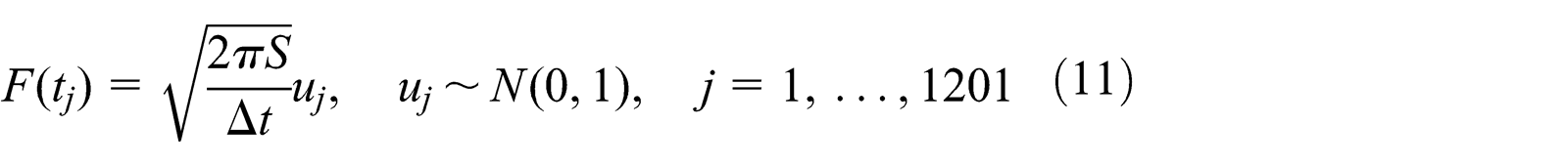
where u_j is an independent standard normal variable and t_j is the jth discrete time step such that t_j = (j−1)Δt. The failure event is defined as the displacement of the oscillator at t ₀ (t ₀ = 12 s) exceeding a prescribed threshold b (b = 0.7 m). Then, the limit state function is defined as follows

$$G(\mathit{u})=b-r(\mathit{u},t_0)$$

(12)

where u is a vector of 1201-D independent normal variables. The design point of this problem is determined by analytical method proposed by Koo et al., ¹⁸ where the design point excitation is identical to the mirror-image excitation f _I(t). In this case

$$f_{\mathrm{I}}(t)=-2c{\stackrel{·}{r}}_{\mathrm{F}}(12-t)$$

(13)

where r _F(t) denotes the free-vibration response of the oscillator, that is, the solution of equation (10) with the right-hand side set to zero and with initial conditions r _F(0) = b. Figure 1 shows the design point of this problem.

Figure 1.

The coordinate value of design point for linear Duffing oscillator subjected to white-noise input.

Generate N (N = 10,000) samples in the 1201-D standard normal space, and the polar features of each sample are calculated by means of equations (5) and (6). The samples are then mapped to a 2D plot as shown in Figure 2 with their class labels calculated by calling the limit state function (12). It can be seen that there is a visual discrimination between the two classes of samples and the failure class samples are in the upper region of the plot, which is compatible with the conclusion of the study by Hurtado. ¹⁴

Figure 2.

Dimensionality reduction of linear Duffing oscillator reliability problem.

Now consider the nonlinear case with γ = 1 m⁻² and the threshold b is set such that b = 0.8 m. The design point for this problem is shown in Figure 3.

Figure 3.

The coordinate value of design point for nonlinear Duffing oscillator subjected to white-noise input.

Overall, 10,000 samples with class labels are mapped to a 2D plot as shown in Figure 4. The sample clustering disappears and the failure class samples are irregularly distributed in the plot. As the design point is calculated accurately, the existence of an important direction for this specific problem is questionable.

Figure 4.

Dimensionality reduction of nonlinear Duffing oscillator reliability problem.

Existence of important direction

Valdebenito et al. ¹⁷ studied the reliability problem of a nonlinear Duffing oscillator subjected to white noise employing the line sampling method, which is also an advanced simulation method ¹⁹ based on the important direction. It turned out that the performance of line sampling method using 50 lines was really poor, which was expected to be very efficient. In order to investigate the reasons, the behavior of the limit state function along each sampled line was studied. It showed that the value of the limit state function along the sampled lines was not only irregular or scattered, but also chaotic. Then, Valdebenito et al. ¹⁷ guessed that the failure region of this specific problem may be composed by disconnected regions or valleys connected by low probability paths.

The conclusion of the study by Valdebenito et al. ¹⁷ can explain the reason why the sample clustering does not exist in Figure 4, that is, the existence of an important direction for this specific problem is, at least, questionable. As the white noise is discretized and represented in the form of high-dimensional variables, the reliability problem of a nonlinear Duffing oscillator is involved. While for a vibration reliability problem which is not involved, for example, a vibration system whose excitation is defined by the random structure parameters only, the important direction may still exist as well as the sample clustering. Meanwhile, it is not appropriate to use the method proposed in this article if we get the wrong or inaccurate important direction for the samples that have no feature of clustering under this condition. The discussions above mean that the DRM can be applied to vibration reliability problems in the case that the important direction exists and one should pay attention when using it. And a visualization analysis should be conducted to make sure that the samples have the clustering feature for a specific problem.

Vibration reliability

The key of the DRM is the determination of the design point. The closed-form solutions of the design point for vibration reliability problems exist only in a few cases. In order to apply the method to more vibration reliability problems, a general method for determining the design point should be discussed.

iHLRF method considering numerical precision

For given t ₀ and b, the design point of a vibration reliability problem is the solution to the constrained optimization problem in standard normal space

$${\mathit{u}}^{*}(t_0,b)=\arg min\{{\Vert \mathit{u}\Vert }^2:G(\mathit{u},t_0,b)=0\}$$

(14)

iHLRF^15,16,20 method is the most popular algorithm used to solve this problem. In this algorithm, every new point u ⁽ⁿ⁺¹⁾ is determined from the previous point u ⁽ⁿ⁾ as follows

$${\mathit{u}}^{(n+1)}={\mathit{u}}^{(n)}+\lambda \mathit{p}$$

(15)

where n denotes the number of iteration, λ is the step size, and p is the search direction defined as follows

$$\mathit{p}=(\frac{G(\mathit{u})}{\Vert \nabla G(\mathit{u})\Vert }+{\mathit{a}}^{\mathrm{T}}\mathit{u})\mathit{a}-\mathit{u}$$

(16)

where $\nabla G(\mathit{u})$ is the gradient vector and a is defined as follows

$$\mathit{a}=\frac{-\nabla G(\mathit{u})}{\Vert \nabla G(\mathit{u})\Vert }$$

(17)

the step size λ is defined by the Armijo rule as follows

$$m_{\mathrm{A}}\left({\mathit{u}}^{(n+1)}\right)-m_{\mathrm{A}}\left({\mathit{u}}^{(n)}\right)\le \frac{1}{2}\lambda (\nabla m_{\mathrm{A}}{\left({\mathit{u}}^{(n)}\right)}^{\mathrm{T}}\mathit{p})$$

(18)

where m _A(·) is the merit function defined as follows

$$m_{\mathrm{A}}(\mathit{u})=\frac{1}{2}\Vert \mathit{u}{\Vert }^2+c_{\mathrm{p}}|G(\mathit{u})|$$

(19)

where c _p is the penalty parameter and should satisfy

$$c_{{}_{\mathrm{p}}}>\frac{\Vert \mathit{u}\Vert }{\Vert \nabla G(\mathit{u})\Vert }$$

(20)

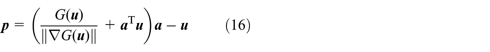
According to the chain rule, the partial derivative of the limit state function with respect to the standardized variable u_i is as follows

$$\frac{\partial G(\mathit{u})}{\partial u_i}=\frac{\partial g(\mathit{x})}{\partial x_i}\frac{\partial x_i}{\partial u_i}=\frac{\partial g(\mathit{x})}{\partial x_i}\frac{\partial {\mathrm{T}}^{-1}(u_i)}{\partial u_i}$$

(21)

where x = ( v , w ) and $\partial g(\mathit{x})/\partial x_i$ is the partial derivative of the limit state function with respect to x . In nonlinear vibration problems, the g( x ) is computed from the numerical integration method. Analytical expressions of the partial derivatives are rarely available and the direct differential method (DDM) can only be applied to a few problems.^21–23 A general program computing the gradient vector often resorts to the finite difference method.^20,24,25

$$\frac{\partial g(\mathit{x})}{\partial x_i}\approx \frac{g(\mathit{x}+\Delta x_i{e}_i)-g(\mathit{x})}{\Delta x_i}$$

(22)

where Δx_i is the perturbation and e _i is the unit vector for the axis x_i .

Theoretically, the truncation error in equation (22) can be reduced using a small perturbation Δx_i . However, the value of the limit state function of nonlinear vibration problem is twofold: one part is deterministic and one part is random, resulting from the computational inaccuracies. It can be reasonably stated that the random part Δg( x ) is proportional to the value of the response itself with a working computational precision imposed by the engineer’s knowledge as the proportionality factor. ²¹ It may lead to a difference g( x +Δx_i e _i)−g( x ) that is smaller than the random part Δg( x ) of the response if the perturbation is too small, which can lead to inaccuracies of the gradient or non-convergence of the iHLRF algorithm. In this article, Δx_i is given by

$${(\Delta x_i)}_{(n)}=q\left|\frac{\Delta g({\mathit{x}}_{(n-1)})}{\nabla g{({\mathit{x}}_{(n-1)})}_i}\right|=q\left|\frac{\mathbf{\epsilon }\mathbf{g}\mathbf{(}{\mathit{x}}_{\mathbf{(}\mathbf{n}\mathbf{-}1\mathbf{)}}\mathbf{)}}{\nabla g{({\mathit{x}}_{(n-1)})}_i}\right|$$

(23)

where q is a magnifying factor, ε is the computational precision, εg( x _(n−1)) is the maximal numerical inaccuracy of the limit state function, and $\nabla g{({\mathit{x}}_{(n-1)})}_i$ is the ith component of the gradient vector at the previous iteration (n−1). The computational precision is stated according to the features of the limit state function.

Reliability

Once the design point has been determined, the DRM can be used to calculate the reliability of vibration systems. But initially, the samples will appear in the plot without the labels safe and failure which can distinguish them only when the limit state function has been called. In this article, a straight line is used to distinguish the two kinds of samples. The preliminary position of the straight line is defined by experience, ²⁶ that is, for low d, the straight line is located in the upper-right sector and titled to the right, while for moderate or high d the line should be close to horizontal. The final position of the straight line is determined after calculating the labels of several samples nearby the initial line and then the samples above the straight line are considered to be failure class. Figure 5 shows the adjustment strategy of the straight line. The dotted line is the initial line and the full line is the final line. The arrows in the figure show the sequence of the samples to be calculated.

Figure 5.

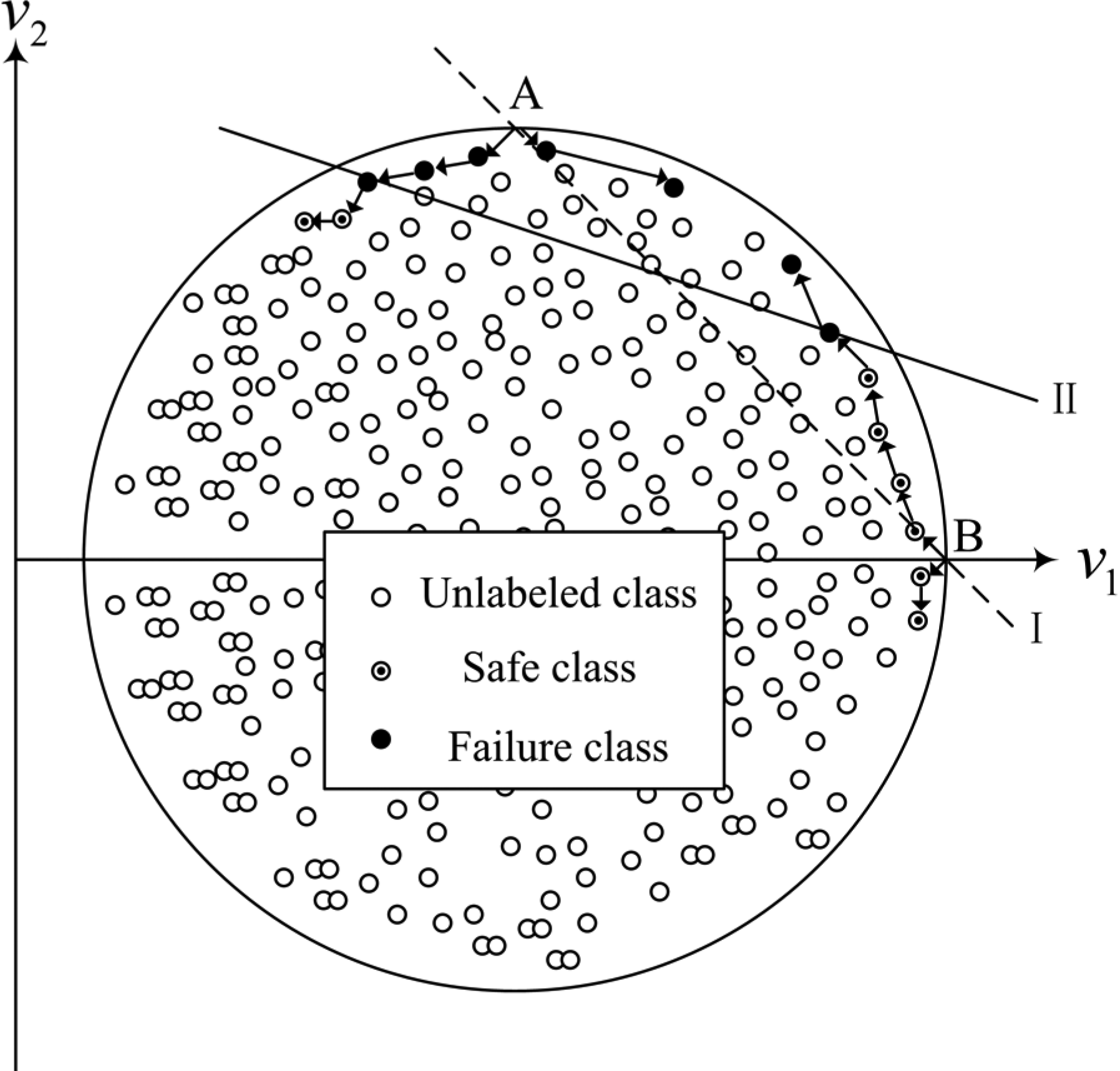
Schematic plot for adjustment strategy of straight line.

The failure probability P _f is calculated by counting the number N _up of the samples above the line

$$P_{\mathrm{f}}=\frac{N_{\mathrm{up}}}{N}$$

(24)

and the reliability is as follows

$$R=1-P_{\mathrm{f}}$$

(25)

It is worth nothing that in the case the important direction does not exist, the DRM cannot be employed to calculate the reliability for that the failure class samples have no characteristics of clustering. But the existence of the sample clustering can be predicted simply by calculating the labels of several samples nearby the initial line.

Numerical example

Consider a single degree-of-freedom impacting system subjected to a horizontal acceleration $\stackrel{··}{y}(t)$ as shown in Figure 6

$$\stackrel{··}{y}(t)=-20t+100\mathrm{cm}/{\mathrm{s}}^2$$

(26)

Figure 6.

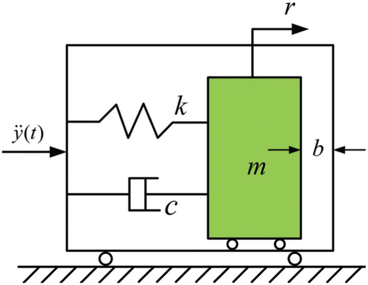
System model of single degree-of-freedom impacting system with strong nonlinearity.

there is a gap b between the mass m and the case wall. The stochastic differential equation is represented by

$$m\stackrel{··}{r}+c\stackrel{·}{r}+k(r+\gamma r^3)=m\stackrel{··}{y}(t)$$

(27)

with initial conditions $r(0)=0$ , $\stackrel{·}{r}(0)=0$ , and m, c, k are independent normal variables. The distribution parameters are set such that µ_m = 10 kg, σ_m = 0.54 kg, µ_c = 10 N s/cm, σ_c = 0.54 N s/cm, µ_k = 30 N/cm, and σ_k = 1.62 N/cm. The failure event is defined as that the mass m impacts on the case wall in 10 s. The deterministic parameters b and γ are set such that b = 0.54 cm and γ = 1000. Then, the limit state function for this problem can be defined as follows

$$g(\mathit{x})=b-r_{max}(\mathit{x},t)$$

(28)

where r _max( x , t) is a function that computes the maximum displacement in a period of time t. All the theories above relate to this kind of reliability problem and the DRM can also be employed.

The original variables x are transformed to standard normal variables by Rosenblatt transformation and the design point is calculated by iHLRF algorithm. In this problem, the use of a fixed perturbation leads to non-convergence of the algorithm, which is due to the fact that the estimation of the gradient vector results in inaccuracy. The design point u ^* = (3.210, 1.496, −2.714) was found after five iterations of the iHLRF algorithm using the perturbation suggested by equation (23). Generate N (N = 10000) samples in the three-dimensional (3D) standard normal space and then map them to the 2D plot. The straight line that separates the two classes of samples is determined by calling the limit state function 22 times. Figure 7 shows the straight line and the samples above it.

Figure 7.

Straight line that separates the two classes of samples and samples above it.

There are 11 samples above the line; thus, the failure probability P _f = N _up/N = 0.0011. Table 1 shows the results of failure probability calculated by FORM, important sampling method (ISM), DRM, and MCM. N _s is the number of samples, N _c is the total number of calls of limit state function to calculate the reliability, P _f is the failure probability, and ${\epsilon }_{P_{\mathrm{f}}}$ is the percentage error in comparison with the standard reference result of MCM.

Table 1.

Results of failure probability.

Algorithm	N s	N c	P f	${\epsilon }_{P_{\mathrm{f}}}$ (%)
MCM	105	105	0.0011	–
FORM	–	221	0.0006	45.45
ISM	1.5×103	1500+221	0.0015	36.36
DRM	104	221+22	0.0011	0

There are only three normal variables in this problem, but the system shows an extreme behavior because of the large value of γ. The reason for the poor performance of FORM is that the approximation of limit state function by a hyperplane is not appropriate due to the strong nonlinearity of the system. The ISM generates an estimator with sufficient accuracy but the numerical cost of the method is relatively high. The DRM almost has the same accuracy as MCM, which is also the most efficient. A visualization analysis is conducted to examine the existence of important direction for this reliability problem. Figure 8 shows that several samples above the straight line are all failure class, which indicates that the important direction exists and the result of design point vector is correct.

Figure 8.

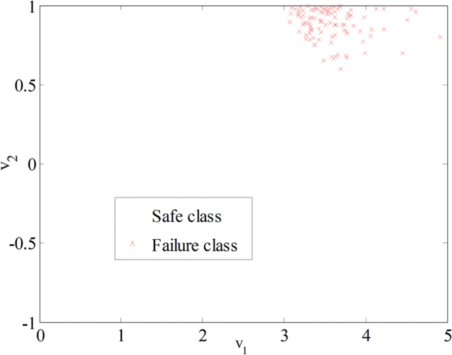
Visualization analysis of single degree-of-freedom impacting reliability problem.

Reliability sensitivity

For vibration systems with uncertain structural parameters, it is important to study the sensitivity of the reliability with respect to the distribution parameters of the uncertainties, such as mean value and standard variance. The reliability sensitivity analysis can help the designer to establish acceptable parameters value, determine the fluctuation of the structural parameters, and select acceptable tolerances.

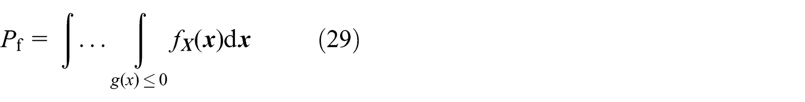
The failure probability of a vibration system is defined as

$$P_{\mathrm{f}}=\int \dots \underset{g(x)\le 0}{\int }{f}_{\mathit{X}}(\mathit{x})\mathrm{d}\mathit{x}$$

(29)

where f _X ( x ) is the joint density function of the original variables x , and the reliability sensitivity is as follows

$$\frac{\partial R}{\partial {\theta }_{x_i}^{(h)}}=-\frac{\partial P_{\mathrm{f}}}{\partial {\theta }_{x_i}^{(h)}}=-\int \dots \underset{g(x)\le 0}{\int }\frac{\partial f_{\mathit{X}}(\mathit{x})}{\partial {\theta }_{x_i}^{(h)}}\mathrm{d}\mathit{x}$$

(30)

where ${\theta }_{x_i}^{(h)}$ is the distribution parameter of the original parameter x_i, i = 1, 2, ...d, and it denotes the mean value when h = 1 and the standard variance when h = 2. Equation (30) is transformed into the form of mathematical expectations as follows

$$\begin{array}{c}\multicolumn{1}{c}{\frac{\partial R}{\partial {\theta }_{x_i}^{(h)}}=-\int \cdots \underset{g(x)\le 0}{\int }\frac{\partial f_{\mathit{X}}(\mathit{x})}{\partial {\theta }_{x_i}^{(h)}}\frac{1}{f_{\mathit{X}}(\mathit{x})}{f}_{\mathit{X}}(\mathit{x})\mathrm{d}\mathit{x}}\\ \multicolumn{1}{c}{\begin{array}{c}\hfill =\hfill \end{array}-\int \cdots \underset{R^d}{\int }{I}_{\mathrm{f}}(\mathit{x})\frac{\partial f_{\mathit{X}}(\mathit{x})}{\partial {\theta }_{x_i}^{(h)}}\frac{1}{f_{\mathit{X}}(\mathit{x})}{f}_{\mathit{X}}(\mathit{x})\mathrm{d}\mathit{x}}\\ \multicolumn{1}{c}{\begin{array}{c}\hfill =\hfill \end{array}-E\left[\frac{I_{\mathrm{f}}(\mathit{x})}{f_{\mathit{X}}(\mathit{x})}\frac{\partial f_{\mathit{X}}(\mathit{x})}{\partial {\theta }_{x_i}^{(h)}}\right]}\end{array}$$

(31)

where I _f( x ) is the indicator function of failure event. According to the mathematical statistics theory, the sample mean value is an unbiased estimate of the population mean value. Then, the reliability sensitivity can be estimated as follows

$$\frac{\partial R}{\partial {\theta }_{x_i}^{(h)}}=-\frac{1}{N}\sum _{j=1}^N\frac{I_{\mathrm{f}}(\mathit{x})}{f_{\mathit{X}}(\mathit{x})}{\frac{\partial f_{\mathit{X}}(\mathit{x})}{\partial {\theta }_{x_i}^{(h)}}|}_{\mathit{x}={\mathit{x}}_j}$$

(32)

where x _j is the jth sample among the N samples generated according to the joint density function of the original variables x . As the samples down the straight line in the 2D plot are considered to be the safe class, the value of their indicator function is equal to zero. Then, equation (32) can be expressed as

$$\frac{\partial R}{\partial {\theta }_{x_i}^{(h)}}=-\frac{1}{N}\sum _{h=1}^{N_{\mathrm{up}}}\frac{1}{f_{\mathit{X}}(\mathit{x})}{\frac{\partial f_{\mathit{X}}(\mathit{x})}{\partial {\theta }_{x_i}^{(h)}}|}_{\mathit{x}={\mathit{x}}_j}$$

(33)

where x _j is the jth sample among the N _up samples which are considered to be failure class.

Numerical example

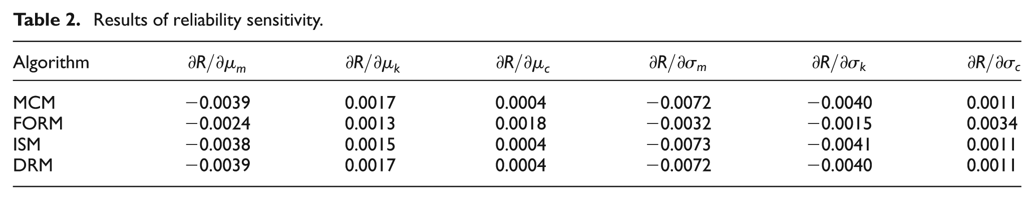
The method is first applied to the single degree-of-freedom impacting system with strong nonlinearity in subsection “Numerical example” of section “Vibration reliability.”Table 2 lists the results of reliability sensitivity calculated by FORM, ISM, and DRM. All the algorithms above will utilize the information provided by the design point result. The results indicate that DRM has the same accuracy as MCM while it deals with a random vibration reliability problem with strong nonlinearity.

Table 2.

Results of reliability sensitivity.

Algorithm	$\partial R/\partial {\mu }_m$	$\partial R/\partial {\mu }_k$	$\partial R/\partial {\mu }_c$	$\partial R/\partial {\sigma }_m$	$\partial R/\partial {\sigma }_k$	$\partial R/\partial {\sigma }_c$
MCM	−0.0039	0.0017	0.0004	−0.0072	−0.0040	0.0011
FORM	−0.0024	0.0013	0.0018	−0.0032	−0.0015	0.0034
ISM	−0.0038	0.0015	0.0004	−0.0073	−0.0041	0.0011
DRM	−0.0039	0.0017	0.0004	−0.0072	−0.0040	0.0011

Then, the example in subsection “Numerical example” of section “Vibration reliability” is extended to a multiple degree-of-freedom impacting system with moderate dimensionality as shown in Figure 9. The horizontal acceleration is as follows

$$\stackrel{··}{y}(t)=-20t+20\mathrm{cm}/{\mathrm{s}}^2$$

(34)

Figure 9.

System model of multiple degree-of-freedom impacting system with moderate dimensionality.

the gap between the mass m ₃ and the case wall is set such that b = 7.2 cm and the nonlinearity of the system is set such that γ = 1. Uncertain parameters for the system are m ₁, m ₂, m ₃, k ₁, k ₂, k ₃, c ₁, c ₂, and c ₃. Each parameter follows a normal distribution and the distribution parameters are listed in Table 3.

Table 3.

Mean value and standard deviation of random variables.

Variables	Distribution type	Mean value	Standard deviation
m 1	Normal	5	0.54
m 2	Normal	6	0.65
m 3	Normal	7.2	0.78
k 1	Normal	10	1.62
k 2	Normal	20	3.24
k 3	Normal	40	6.48
c 1	Normal	10	0.54
c 2	Normal	15	0.81
c 3	Normal	23	0.98

The failure event is defined as that the mass m ₃ impacts on the case wall in 10 s. The design point for this problem is that u ^* = (1.088, −0.156, 1.019, −2.769, −0.096, 0.297, −0.589, 0.511, 0.002). Generate N (N = 10,000) samples in the nine-dimensional (9D) standard normal space and then map them to the 2D plot. Figure 10 shows the straight line that separates the two classes of samples and the samples above it. A visualization analysis is conducted to examine the existence of important direction for this reliability problem. Figure 11 shows that several samples above the straight line are all failure class, which indicates that the important direction exists and the result of design point vector is correct.

Figure 10.

Straight line that separates the two classes of samples and samples above it.

Figure 11.

Visualization analysis of multiple degree-of-freedom impacting reliability problem.

There are 36 samples above the straight line; thus, the reliability R = 1−N _up/N = 0.9964. As the reliability sensitivity analysis requires the position of the failure samples, the ability of capturing the failure samples of different algorithms is compared by calculating the failure probability and the results are listed in Table 4. N _c is the total number of calls of limit state function to calculate the failure probability, P _f is the failure probability, and the result of MCM is used as the standard reference. The result calculated by DRM shows good accuracy and it requires less number of calls of limit state function, which indicates that the DRM has good capacity of capturing the failure samples. The reliability sensitivity is calculated by equation (33) using the position of the failure class samples in the original space corresponding to the samples above the straight line in the 2D plot. The results of reliability sensitivity are as follows

$$\frac{\partial R}{\partial \mathbf{\mu }}={\left[\begin{array}{c}\hfill \partial R/\partial {\mu }_{m_1}\hfill \\ \multicolumn{1}{c}{\partial R/\partial {\mu }_{m_2}}\\ \multicolumn{1}{c}{\partial R/\partial {\mu }_{m_3}}\\ \multicolumn{1}{c}{\partial R/\partial {\mu }_{k_1}}\\ \multicolumn{1}{c}{\partial R/\partial {\mu }_{k_2}}\\ \multicolumn{1}{c}{\partial R/\partial {\mu }_{k_3}}\\ \multicolumn{1}{c}{\partial R/\partial {\mu }_{c_1}}\\ \multicolumn{1}{c}{\partial R/\partial {\mu }_{c_2}}\\ \multicolumn{1}{c}{\partial R/\partial {\mu }_{c_3}}\end{array}\right]}^{\mathrm{T}}={\left[\begin{array}{c}\hfill -0.00454\hfill \\ \multicolumn{1}{c}{-0.00571}\\ \multicolumn{1}{c}{-0.00683}\\ \multicolumn{1}{c}{0.00575}\\ \multicolumn{1}{c}{0.00131}\\ \multicolumn{1}{c}{0.00037}\\ \multicolumn{1}{c}{0.00158}\\ \multicolumn{1}{c}{0.00118}\\ \multicolumn{1}{c}{0.00042}\end{array}\right]}^{\mathrm{T}},\frac{\partial R}{\partial \mathbf{\sigma }}={\left[\begin{array}{c}\hfill \partial R/\partial {\sigma }_{m_1}\hfill \\ \multicolumn{1}{c}{\partial R/\partial {\sigma }_{m_2}}\\ \multicolumn{1}{c}{\partial R/\partial {\sigma }_{m_3}}\\ \multicolumn{1}{c}{\partial R/\partial {\sigma }_{k_1}}\\ \multicolumn{1}{c}{\partial R/\partial {\sigma }_{k_2}}\\ \multicolumn{1}{c}{\partial R/\partial {\sigma }_{k_3}}\\ \multicolumn{1}{c}{\partial R/\partial {\sigma }_{c_1}}\\ \multicolumn{1}{c}{\partial R/\partial {\sigma }_{c_2}}\\ \multicolumn{1}{c}{\partial R/\partial {\sigma }_{c_3}}\end{array}\right]}^{\mathrm{T}}={\left[\begin{array}{c}\hfill -0.00263\hfill \\ \multicolumn{1}{c}{-0.00412}\\ \multicolumn{1}{c}{-0.00709}\\ \multicolumn{1}{c}{-0.01147}\\ \multicolumn{1}{c}{-0.00141}\\ \multicolumn{1}{c}{-0.00029}\\ \multicolumn{1}{c}{0.00006}\\ \multicolumn{1}{c}{-0.00082}\\ \multicolumn{1}{c}{-0.00031}\end{array}\right]}^{\mathrm{T}}$$

(35)

Table 4.

Failure probability of different methods.

Algorithm	N s	N c	P f	${\epsilon }_{P_{\mathrm{f}}}$ (%)
MCM	105	105	0.0035	–
FORM	–	186	0.0006	82.86
ISM	1.5×103	186+1500	0.0036	2.86
DRM	104	186+32	0.0036	2.86

As the effects of design parameters on reliability of general system are different, it is important to know the influence of random parameters. Because of the difference of parameter dimension, it is difficult to obtain the comparison results for reliability sensitivity of statistical characteristic, so the results of reliability sensitivity must be non-dimensional-normalized. The standard deviation is used as a normalization factor to make the sensitivity measures dimensionless and more appropriate for variable ranking.^27,28 The non-dimensional reliability sensitivity can be expressed as

$$S_{\mathrm{non}}({\mu }_x)=\frac{\partial R/R}{\partial {\mu }_x/{\sigma }_x}$$

(36)

$$S_{\mathrm{non}}({\sigma }_x)=\frac{\partial R/R}{\partial {\sigma }_x/{\sigma }_x}$$

(37)

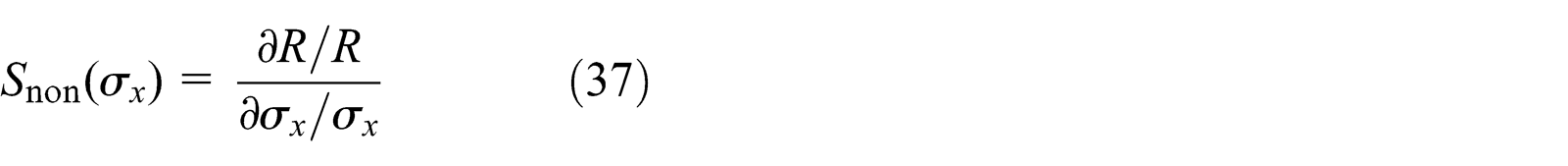
where S _non(µ_x ) is the non-dimensional reliability sensitivity with respect to the mean value of random parameter; S _non(σ_x ) is the non-dimensional reliability sensitivity with respect to the standard deviation of random parameter. Then, the sensitivity factor S _f of each random variable is defined as follows

$$S_{\mathrm{f}}(\mathrm{x})=\sqrt{S_{\mathrm{non}}^2({\mu }_x)+S_{\mathrm{non}}^2({\sigma }_x)}$$

(38)

Figure 12 shows the non-dimensional reliability sensitivity result and the proportion plot of each sensitivity factors. It can be found that the non-dimensional reliability sensitivity for the mean value of k ₁, k ₂, k ₃, c ₁, c ₂, and c ₃ are positive, and for the mean value of m ₁, m ₂, and m ₃ and the variance of m ₁, m ₂, m ₃, k ₁, k ₂, k ₃, c ₁, c ₂, and c ₃ are negative. That is to say the reliability of the vibration system increases as the mean value of k ₁, k ₂, k ₃, c ₁, c ₂, and c ₃ increases, but descends as the mean value of m ₁, m ₂, and m ₃ and the variance of m ₁, m ₂, m ₃, k ₁, k ₂, k ₃, c ₁, c ₂, and c ₃ increases. The sensitivity factors of the structural parameters in the order of degree of influence on reliability are k ₁, m ₃, k ₂, m ₂, m ₁, k _3, c ₁, c ₂, and c ₃. The polar transformation-based reliability sensitivity analysis method is very efficient to solve reliability and reliability sensitivity problems of vibration systems almost with the same accuracy as the MCM, which in the absence of analytical solutions is the standard reference for accuracy in this field.

Figure 12.

Non-dimensional reliability sensitivity and the proportion plot of each sensitivity factors: (a) non-dimensional reliability sensitivity with respect to mean value, (b) non-dimensional reliability sensitivity with respect to standard deviation, and (c) proportion plot of each sensitivity factors.

Conclusion

In this article, the DRM was applied to vibration reliability and reliability sensitivity problems and the applicability of the method was investigated. The study of the Duffing oscillator subjected to white noise shows that in the case the important direction of a reliability problem does not exit, the application is inappropriate. In order to apply the method to more vibration reliability problems, the iHLRF method was modified when calculating the design point. The reliability of a single degree-of-freedom impacting system was calculated, and the influence of structural parameters on the reliability of a multiple degree-of-freedom impacting system was studied. Numerical results were presented.