Sage Journals: Discover world-class research

Abstract

A systematic research of steady state for the dynamic job shop scheduling problem with jobs releasing continuously over time has been conducted in this article. A simulation scheduling test for the purpose of factor analysis is designed and carried out first and then another simulation scheduling test for the purposes of disciplinarian investigation is conducted. The heuristic dispatching rule algorithm is adopted in the simulation scheduling. The test data are processed and analyzed using SPSS13.0. The results indicated that the dominant factor that can characterize the shop steady state is the shop utilization level. Besides, the relationship between the number of jobs arrived at the shop and the steady state of the shop can be described by a quadratic curve preferably. Results obtained in this article make significant sense for the study of simulation scheduling of dynamic job shop scheduling problem and also for the optimum design of the shop system.

Keywords

Dynamic job shop scheduling problem steady state of shop simulation scheduling heuristic dispatching rule algorithm

Introduction

The job shop scheduling problem (JSP) is one of the most important problems in manufacturing informatization and automation technology, and it is also an important research topic in advanced manufacturing technology and one of the hot issues in operations research. The semantic description of classical JSP in manufacturing systems can be stated as follows: there are n different jobs waiting to be processed in a shop that includes m different machines. Each job consists of a set of operations, and the operation sequence on each machine is prespecified. Each operation is characterized by a specified machine and a fixed period of processing time. Different jobs consist of different operations and operation sequences. The objective is to find out processing sequences on each machine which can make the performance measures related to the manufacturing system achieve optimal or near optimal while satisfying the conditions mentioned above.

The JSP can be divided into static and dynamic JSPs according to the scheduling environment. The classical JSP usually consists of a series of assumptions, such as all jobs arrive at the shop simultaneously, no preemption is allowed and no machine failures occur during the processing time, and the buffer is infinite, so it belongs to the static JSP. However, the static JSP is not consistent with most of the practical scheduling problems in the manufacturing system. Therefore, many scholars and engineering researchers put forward some extensions on the basis of the classical JSP, such as taking the machine failure into account and the jobs arrived at the shop continuously instead of simultaneously, and this kind of problem is often called dynamic JSP.¹ In many practical manufacturing systems, the jobs arrived at the shop in succession. Much more is this the case in the order-oriented manufacturing system. Therefore, it is important to give consideration to the dynamic JSP. In this article, we discussed the dynamic JSP in which the jobs arrived continuously over time and explored the steady state of the shop in simulation scheduling that aims at providing the basis for the critical technical key points in solving such kind of problems.

Simulation scheduling and steady state of shop

Algorithms for solving JSP are usually divided into two broad categories: accurate algorithms and approximate algorithms. Accurate algorithms, such as mathematical programming methods² and branch-and-bound method,^3,4 can only be used effectively in some simple and small-scale scheduling problems. Approximate algorithms include genetic algorithm,⁵ ant colony algorithm,⁶ particle swarm optimization algorithm,^7,8 simulated annealing algorithm,^9,10 tabu search algorithm,¹¹ other intelligent algorithms,¹² and heuristic priority rule¹³ algorithms. Approximate algorithms have been widely used to solve the scheduling problems, although usually they cannot obtain the global optimal solution, but with less complexity and cost to obtain the near-optimal scheduling schemes to meet the actual requirements, they are also a hot spot in algorithm research in recent years.

Studies on JSPs in which jobs arrive at the shop continuously over time, that is, the dynamic JSP, is increasing. The effective algorithm for solving this kind of problem is the heuristic priority rules in which the selection and design are critical. Different scheduling rules lead to different scheduling schemes and directly affect the performance of the scheduling scheme. The greatest advantage of heuristic priority rules lies in its adaptation to the constructive of the dynamic job arrivals, algorithms of low complexity, and its rapid response. However, the biggest disadvantage of dispatching rule is that it depends on the characteristics of scheduling problems seriously. There is no mathematical analysis as criterion for the relationship between dispatching rules and scheduling models or scheduling objectives so far.

Blackstone et al.¹⁴ mention that the study of job shops by analytic techniques, such as queuing theory, becomes extremely complex even for small-scale problems. Therefore, the use of simulation for analyzing this problem is unavoidable. Due to the same difficulty in examining the heuristic algorithms for solving dynamic job shop scheduling problems (DJSPs), we also rely on simulation to study the problem. The method of simulation scheduling for testing the dynamic JSP has the advantage of ease implementation and cost saving in justifying the validity of approaches. But its biggest shortcoming lies in that it does not have the universality which means that when a small change occurred in the scheduling scenario, the conclusions obtained before cannot be adapted to the new situation, so the results drawn through simulation scheduling are vulnerable to the influence of disturbance. Overall, simulation scheduling test on dynamic JSP is the most effective method, and it was widely used by scholars and researchers at home and abroad in dealing with the problem of dynamic JSP.

As a virtual test procedure, simulation scheduling includes two key segments: experimental design and the processing and analysis of the experimental results. In addition, the key points of design techniques for the simulation scheduling test include two aspects: the generation of the scheduling test data and the determination of the test parameters. In the simulation scheduling test, the main parameters are the number of simulation runs (equivalent to the number of samples), the number of jobs in each simulation (equivalent to the length of the samples), and the start sampling point.

In the simulation of JSP in which jobs arrive continuously, it is usually assumed that all machines in the shop are idle in the initial state and then jobs arrive at the shop according to a certain probability distribution of time intervals. It is clear that the shop utilization level (or shop load level) is slightly lower in the initial stage, and it will gradually rise as the jobs continuously arrive. After a certain period of time, that is, after a certain number of jobs arrived, the state of the shop tends to be dynamic steady, along with the shop utilization level and other shop indexes.

In the experimental study of simulation scheduling, sampling usually begins when the shop reaches a steady state, that is, the time the shop reaches the steady state as a starting point for sampling so as to make the experimental data statistically meaningful. In the simulation scheduling section of the literature,¹⁵ all jobs arrived at the shop continuously, and samples were in batches which included 1000 jobs in each batch. The article pointed out that the first batch of 1000 jobs corresponding to the sampling point should be deleted, so that the start sampling point was 1001, which means that the shop reaches a steady state from the second batch. In the literature,^16–19 several shop parameters (such as shop utilization level and the average flow time of job) during the scheduling process were observed to determine the time when the shop reached the steady state, and the result indicated that the shop reached steady state after 500 jobs arrived at the shop. Then, the literature²⁰ showed that it was after 250 jobs arrived at the shop that the shop reached steady state. The simulation scheduling in Sha et al.²¹ was calculated by the unit of days in which the sampling data were from the 151th after 150 days of preheating, which means that the 150th day was regarded as the starting point of steady state. As can be seen, the findings of the literatures mentioned above were varying, and there are no detailed data and analysis to support the results. In this article, we tried to explore the time the shop reaches steady state in simulation scheduling for the purpose of solving this kind of problem more accurately and effectively in future.

Design of simulation scheduling experiment

This article studied the dynamic JSP using the priority dispatching rules. Simulation scheduling was conducted with the configuration of different shop scheduling system parameters to investigate the factors that can represent the steady state of the shop and the arrival time (or the corresponding number of jobs) the shop reaches the steady state. The literature²² indicated that the shop utilization level, the number of operations of jobs, and their processing times would affect the performance of the shop in a certain extent, whereas other parameters such as the number of machines and the distribution of job arrival time would not.

The model framework of the dynamic JSP is as follows: there are 10 machines in the shop; jobs arrive at the shop by the time interval of exponential distribution; the number of operations of each job and the processing time of each operation is generated according to the discrete uniform distribution; the operations of the same job has precedence constraints; and the processing machine of each operation is selected randomly in 10 machines in probability way, but the processing machine for each operation is unique and the processing machine for the adjacent operation of the same job is different.

In order to study the steady state of the dynamic job shop scheduling systematically, the scheduling experiments were performed in two steps. First, different model instances were obtained by configuring different parameter sets according to the model framework. By doing so, the factors influence the steady state of the shop and its influencing degree is explored through results processing and analyzing. In addition, the main influencing factors were found out, and the exploration of their influence trends and the law were summarized.

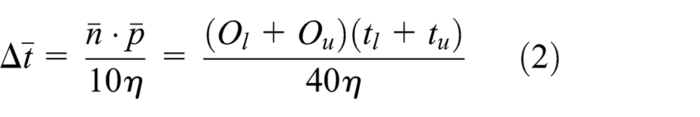
The structure of the parameter set for the model instance is as follows

Ω_{i} = {η, {O_{l}, O_{u}}, {t_{l}, t_{u}}}

(1)

where $Ω_{i}$ is a certain set of numbers; $η$ is the shop utilization level; $O_{l}$ and $O_{u}$ are the lower and upper bounds of the uniform distribution that contains the number of operations for the jobs, respectively; and $t_{l}$ and $t_{u}$ are the lower and upper limits of the discrete uniform distribution for the operation processing time, respectively.

Let $\bar{p}$ denotes the average processing time of the operation and $\bar{n}$ denotes the average number of job operations, so the mean interval time for the continuously arrived jobs $Δ \bar{t}$ can be obtained by the following formula

Δ \bar{t} = \frac{\bar{n} \cdot \bar{p}}{10 η} = \frac{(O_{l} + O_{u}) (t_{l} + t_{u})}{40 η}

(2)

And the interval time for the continuously arrived jobs can be obtained by the following equation

Δ t = - Δ \bar{t} \cdot \ln \tilde{r}

(3)

where $\tilde{r}$ is a random number between 0 and 1.

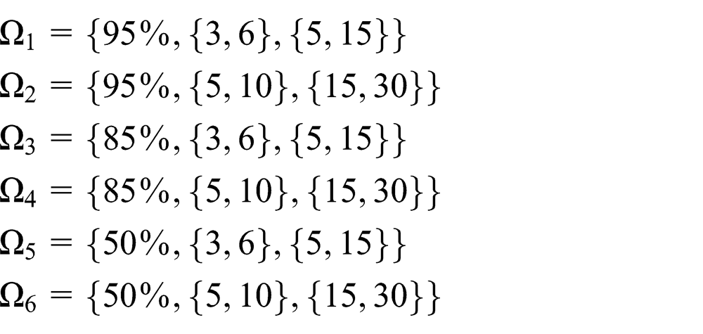
The parameter sets for the first step of scheduling experiment are as follows

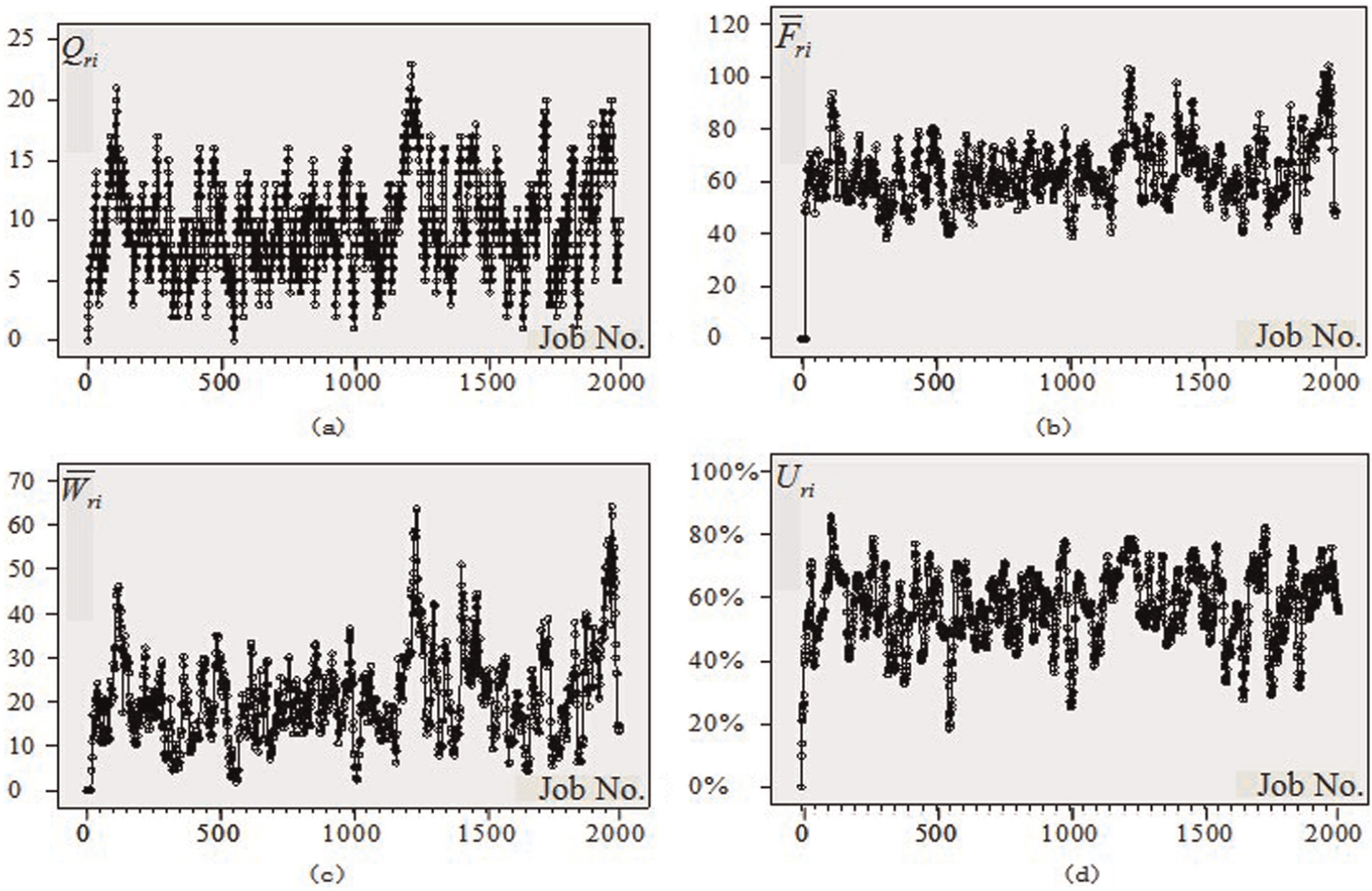
\begin{matrix} Ω_{1} = {95 %, {3, 6}, {5, 15}} \\ Ω_{2} = {95 %, {5, 10}, {15, 30}} \\ Ω_{3} = {85 %, {3, 6}, {5, 15}} \\ Ω_{4} = {85 %, {5, 10}, {15, 30}} \\ Ω_{5} = {50 %, {3, 6}, {5, 15}} \\ Ω_{6} = {50 %, {5, 10}, {15, 30}} \end{matrix}

The scheduling experiment was run 10 times under each parameter set, and the samples obtained through the 10 experiments were independent and identically distributed in a sense of probability because they shared the same parameter set and model. The samples for each run were obtained in the way of point sampling mode, that is, sampling was carried out each time a job arrived at the shop. The sampling length is 2000, that is, 2000 jobs would arrive at the shop. In order to evaluate the steady state of the shop, four indicators, namely, the work in process inventory, the average flow time of the job, the average waiting time of the job, and the real-time shop utilization level, were taken as sample observations.

The design of the parameter set for the second step of the scheduling experiment is based on the results of the first step. The influencing trend and law are studied through the refinement of the parameters corresponding to the main influence factors while keeping other parameters constant.

The algorithm for the dynamic scheduling is the heuristic dispatching rule,²³ and the scheduling rule is operation due date (ODD), that is, priority is given to the operation with the smallest remained completion time.

Analysis of the simulation scheduling experiment

Results of simulation scheduling experiment

Experiment data processing

The results of the scheduling experiment can be processed according to the following procedures:

Let $O_{ri}$ denote the ith observation value of the rth time running, and $Q_{ri}$ , ${\bar{F}}_{ri}$ , ${\bar{W}}_{ri}$ , and $U_{ri}$ denote the four indicators, namely, the work in process inventory, the average flow time of the job, the average waiting time of the job, and the real-time shop utilization level, respectively, so we have

\begin{matrix} O_{ri} \in (Q_{ri}, {\bar{F}}_{ri}, {\bar{W}}_{ri}, U_{ri}) r = 1, 2, \dots, 10; \\ i = 1, 2, \dots, 2000 \end{matrix}

(4)

For the 10 ensemble average that belong to each parameter set

{\bar{O}}_{• i} = \frac{1}{10} \sum_{r = 1}^{10} O_{ri}, i = 1, 2, \dots, 2000

(5)

Take the job arrival order i as the independent variable and the ensemble average ${\bar{O}}_{• i}$ as the dependent variable to draw scatter diagrams. As the jobs continuously arrive, the tendency of each index can be observed to evaluate the trend of the state of the shop.

Results of simulation scheduling experiment

The job number–ensemble average diagram was obtained by independent development of the Java application program, according to the scheduling method in the literature.⁹

Effects of shop utilization level. The simulation scheduling was performed under three parameter sets, namely, $Ω_{1}$ , $Ω_{3}$ , and $Ω_{5}$ , and the results were processed by the method mentioned above. The scatter diagrams are shown in Figures 1 –3.

Effects of the number of operations and operation processing time. The combination of the number of operations and processing time for the job operations can directly reflect the influence on the total processing time of jobs, so it was studied as a combination of these factors. Let both the number of operations and operation processing time change under three different shop utilization levels to obtain parameter set $Ω_{2}$ , $Ω_{4}$ , and $Ω_{6}$ . Simulation scheduling was carried out under these three parameter sets, and the processed results are shown in Figures 4 –6.

Figure 1.

Scheduling results under the parameter set of $Ω_{1}$ : (a) $Q_{ri}$ , (b) ${\bar{F}}_{ri}$ , (c) ${\bar{W}}_{ri}$ , and (d) $U_{ri}$ .

Figure 2.

Scheduling results under the parameter set of $Ω_{3}$ : (a) $Q_{ri}$ , (b) ${\bar{F}}_{ri}$ , (c) ${\bar{W}}_{ri}$ , and (d) $U_{ri}$ .

Figure 3.

Scheduling results under the parameter set of $Ω_{5}$ : (a) $Q_{ri}$ , (b) ${\bar{F}}_{ri}$ , (c) ${\bar{W}}_{ri}$ , and (d) $U_{ri}$ .

Figure 4.

Scheduling results under the parameter set of $Ω_{2}$ : (a) $Q_{ri}$ , (b) ${\bar{F}}_{ri}$ , (c) ${\bar{W}}_{ri}$ , and (d) $U_{ri}$ .

Figure 5.

Scheduling results under the parameter set of $Ω_{4}$ : (a) $Q_{ri}$ , (b) ${\bar{F}}_{ri}$ , (c) ${\bar{W}}_{ri}$ , and (d) $U_{ri}$ .

Figure 6.

Scheduling results under the parameter set of $Ω_{6}$ : (a) $Q_{ri}$ , (b) ${\bar{F}}_{ri}$ , (c) ${\bar{W}}_{ri}$ , and (d) $U_{ri}$ .

Analysis of scheduling experiment results

In Figure 1, the trend of the four indicators, namely, the work in process inventory, the average flow time of the job, the average waiting time of the job, and the real-time shop utilization level, is roughly the same for the same parameters set. The trend sharply rises in the initial phase and then becomes stable, but the stability is not so obvious because significant fluctuations exist. At the same time, the phenomenon that the real-time utilization level of the shop from initial suddenly rose to steady is very obvious. Results under other parameter sets also show the same rule.

Comparing the trend of the same indicators under parameter sets of different shop utilization level according to Figures 1 –3, we can draw the conclusion that it is obvious the shop utilization level can be used as an indicator to characterize the steady state of the shop. In Figure 1, when the shop utilization level is set 95%, the shop reaches the steady state slowly, but the shop can quickly reach the steady state when setting the shop utilization level to 50% as shown in Figure 3.

Comparing Figure 1 with Figure 4, Figure 2 with Figure 5, and Figure 3 with Figure 6, we can see that the changing trends of the observation indicator are not so obvious when the number of operations of jobs and operation processing time are different while keeping the shop utilization level as the same. Thus, we can conclude that the indicator that can characterize the steady state of the shop is the shop utilization level.

Research on the influencing trend

Conclusions can be drawn from the previous section that the shop utilization level is the main indicator that can characterize the steady state of the shop. For further study on the influence trend and the rule, we refine the setting of the shop utilization level while keeping the number of job operations and operation processing time constant. The addition of the parameter sets is as follows after refinement

\begin{matrix} Ω_{7} = {75 %, {3, 6}, {5, 15}} \\ Ω_{8} = {65 %, {3, 6}, {5, 15}} \\ Ω_{9} = {40 %, {3, 6}, {5, 15}} \end{matrix}

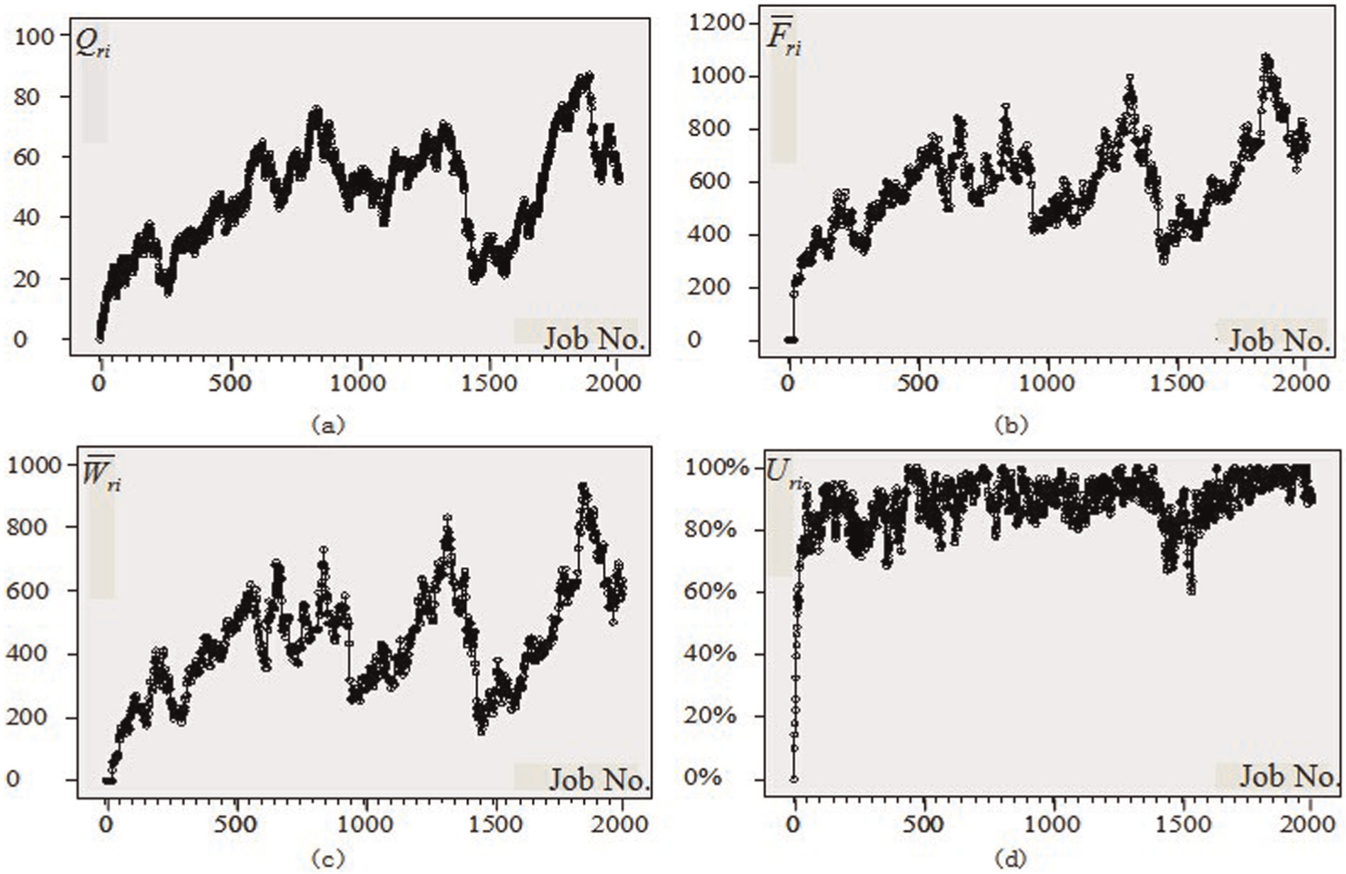
Taken the real-time shop utilization level as the examine indicator, simulation scheduling was carried out under six parameter sets, namely, $Ω_{1}$ , $Ω_{3}$ , $Ω_{5}$ , $Ω_{7}$ , $Ω_{8}$ , and $Ω_{9}$ . The experimental results are shown in Figures 7 –12.

Figure 7.

Real-time shop utilization level under parameter set $Ω_{1}$ .

Figure 8.

Real-time shop utilization level under parameter set $Ω_{3}$ .

Figure 9.

Real-time shop utilization level under parameter set $Ω_{7}$ .

Figure 10.

Real-time shop utilization level under parameter set $Ω_{8}$ .

Figure 11.

Real-time shop utilization level under parameter set $Ω_{5}$ .

Figure 12.

Real-time shop utilization level under parameter set $Ω_{9}$ .

From Figures 7 –12, we can see that when the shop utilization level decreases, the shop reaches the steady state faster, that is, the lower the shop load level, the faster the shop reaches its steady state. The relationship between the shop utilization level and the number of the jobs arrived at the shop at its steady state is shown in Table 1.

Table 1.

Relationship between the shop utilization level and the number of jobs arrived at the shop at its steady state.

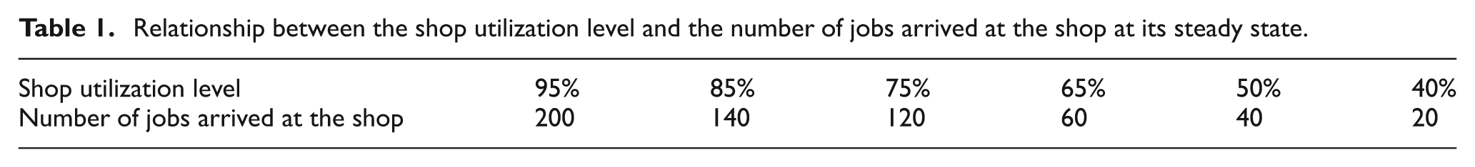
Shop utilization level	95%	85%	75%	65%	50%	40%
Number of jobs arrived at the shop	200	140	120	60	40	20

According to the data in Table 1, curve estimation is conducted for the preselected linear (Linear), the logarithmic curve (Logarithmic), quadratic curve (Quadratic), cubic curve (Cubic), and compound curve (Compound). The fitting results are shown in Table 2.

Table 2.

Fitting results of the curve.

Curve	Item
	Statistical test value					Parameter estimation
	R²	F	df1	df2	Significance	Constant	b1	b2	b3
Linear	0.945	68.198	1	4	0.001	−121.374	3.191
Logarithmic	0.887	31.549	1	4	0.005	−725.160	196.536
Quadratic	0.981872	81.245	2	3	0.00244	46.379	−2.243	0.040
Cubic	0.981778	80.821	2	3	0.00246	−0.057	0.000	0.006	0.000
Compound	0.973	144.340	1	4	0.000	4.494	1.042
Exponential	0.973	144.340	1	4	0.000	4.494	0.041

Conclusions can be drawn from Table 2; the R² determination coefficients of the quadratic curve and cubic curve were the maximum. Among them, the corresponding value of the quadratic curve was larger which demonstrates that its fitting degree was the best. Then, from the significant degree, the fact that the corresponding value of the quadratic curve was smaller than the cubic’s indicated that the parameter estimation of the quadratic curve was more significant. Therefore, the quadratic curve was selected to express the relationship between the setting of the shop utilization level and the number of the jobs arrived at the shop at its steady state

n_{w} = 46.379 - 2.243 η + 0.040 η^{2}

(6)

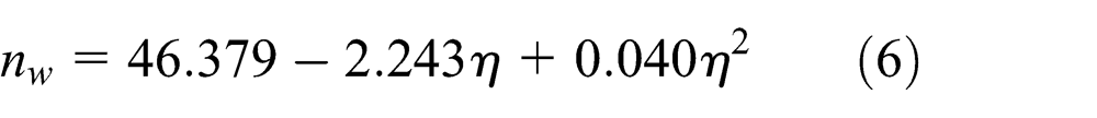
where $η$ is the setting value of the shop utilization level and $n_{w}$ is the number of jobs arrived at the shop at its steady state.

Conclusions can also be drawn from Figures 7 –12, that is, the higher the value of the shop utilization level, the greater the stability under the steady state. And with the decrease in the shop utilization level, the volatility of the shop in steady state increases.

Conclusion and discussion

Conclusion

Simulation scheduling is the main method in studying the dynamic JSP, so data sampling is an important part as a simulation random test. In order to ensure the statistical significance of the data sampling, the start point of sampling (i.e. the number of the jobs arrived at the shop at its steady state) is one of the important factors to consider. From the simulation scheduling and data processing results above, some conclusions can be drawn from it:

Many literatures^15,17 assumed that the number of jobs was 500 when the shop reached its steady state in simulation scheduling, but the systematic simulation scheduling experiments indicated that the number of jobs and the time the shop reaches its steady state were different under different shop parameter sets. However, 500 jobs were large enough to ensure that the shop had already reached its steady state.

When the simulation scheduling was conducted under the same parameter set, the trend of the four indicators, namely, the work in process inventory, the average flow time of the job, the average waiting time of the job, and the real-time shop utilization level, was roughly the same. Among the three parameter sets of the shop utilization level, the number of operations, and the processing time, the influence of the shop utilization level is the most obvious, so it is the main indicator that can characterize the steady state of the shop.

Through curve estimation, the relationship between the shop utilization level and the number of jobs arrived at the shop is quadratic curve. According to the corresponding equation, the number of jobs and the time the shop reaches its steady state under different shop utilization levels can be calculated.

Analysis and discussion

From the standpoint of theoretical study’s significance, the results of the study in this article can provide a theoretical basis for the simulation scheduling of dynamic JSP and avoid blindness in data sampling so as to ensure the rationality of the simulation scheduling results.

In engineering practice, the simulation model of the shop system can be built first among the three cases including the design of the shop system, the matching of optimization resource, and the evaluation of the shop performance. The process and method of simulation scheduling in this article can provide an important and a rational theoretical basis for the building of the simulation model.

The study of the last section in this article aims at the indicator of the real-time shop utilization level. In the research of the classical dynamic job shop scheduling, the indicators that need to optimize usually are the average flow time, the maximum flow time, and other due date–related indicators. The study of the steady state under these indicators can be investigated using the same method and procedures described in this article.

Footnotes

Acknowledgements

The authors would like to express their gratitude to the anonymous reviewers, whose discussion with them was advantageous to improve the quality of this article.

Academic Editor: Duc T Pham

Declaration of conflicting interests

The author(s) declared no potential conflicts of interest with respect to the research, authorship, and/or publication of this article.

Funding

This research was supported by the National Natural Science Foundation of China under grant no. 71271160 and also by Research Foundation of Education Bureau of Hubei Province (China) under grant no. D20121102.

References

Nie

Gao

. A GEP-based reactive scheduling policies constructing approach for dynamic flexible job shop scheduling problem with job release dates. J Intell Manuf 2013; 24: 763–774.

Van Hulle

. A goal programming network for mixed integer linear programming: a case study for the job-shop scheduling problem. Int J Neural Network 1991; 2: 201–209.

Balas

. Machine scheduling via disjunctive graphs: an implicit enumeration algorithm. Oper Res 1969; 17: 941–957.

Carlier

Pinson

. An algorithm for solving the job shop problem. Manage Sci 1989; 35: 164–176.

Zhang

Gao

Shi

. An effective genetic algorithm for the flexible job-shop scheduling problem. Expert Syst Appl 2011; 38: 3563–3573.

Dorigo

Gambardella

. Ant colony system: a cooperative learning approach to the traveling salesman problem. IEEE T Evolut Comput 1997; 1: 53–56.

Kennedy

Eberhart

. Particle swarm optimization. In: Proceedings of IEEE international conference on neutral networks, Perth, WA, Australia, 1995, pp.1942–1948. New York: IEEE.

Gao

Zhou

. PSO based scheduling algorithm for open shop scheduling problem. Chin J Mech Eng 2006; 47: 129–134.

Van Laarhoven

PJM

Aarts

EHL

Lenstra

. Job shop scheduling by simulated annealing. Oper Res 1992; 40: 113–125.

10.

Zhang

Rao

. A new hybrid GA/SA algorithm for the job shop scheduling problem. In: Raidl

Gottlieb

(eds) Evolutionary computation in combinatorial optimization (Lecture notes in computer science, vol. 3448). Berlin, Heidelberg: Springer, 2005, pp.246–259.

11.

Taillard

. Parallel taboo search technique for the jobshop scheduling problem. Technical report ORWP 89/11, DMA, Ecole Polytechnique Fédérale de Lausanne, Lausanne, 1989.

12.

Zhang

Gao

. A hybrid intelligent algorithm and rescheduling technique for job shop scheduling problems with disruptions. Int J Adv Manuf Tech 2013; 65: 1141–1156.

13.

Glover

Greenberg

. New approaches for heuristic search: a bilateral linkage with artificial intelligence. Eur J Oper Res 1989; 39: 119–130.

14.

Blackstone

Philips

Hogg

. A state-of-the-art survey of dispatching rules for manufacturing job shop operations. Int J Prod Res 1982; 20: 27–45.

15.

Rachamadugu

Schriber

. Performance of dispatching rules under perfect sequencing flexibility. In: Proceedings of the 1990 winter simulation conference, New Orleans, LA, 9–12 December 1990, pp.653–658. New York: IEEE.

16.

Holthaus

Rajendran

. Efficient dispatching rules for scheduling in a job shop. Int J Prod Econ 1997; 48: 87–105.

17.

Holthaus

. Scheduling in job shops with machine breakdowns: an experimental study. Comput Ind Eng 1999; 36: 137–162.

18.

Rajendran

Holthaus

. A comparative study of dispatching rules in dynamic flowshops and jobshops. Eur J Oper Res 1999; 116: 156–170.

19.

Mohanasundaram

Natarajan

Viswanathkumar

. Scheduling rule for dynamic shops that manufacture multi-level jobs. Comput Ind Eng 2003; 44: 119–131.

20.

Jayamohan

Rajendran

. Development and analysis of cost-based dispatching rules for job shop scheduling. Eur J Oper Res 2004; 157: 307–321.

21.

Sha

Hsu

Che

. A dispatching rule for photolithography scheduling with an on-line rework strategy. Comput Ind Eng 2006; 50: 233–247.

22.

Ramasesh

. Dynamic job shop scheduling: a survey of simulation research. Omega 1990; 18: 43–57.

23.

Xiong

Kong

. A heuristic method for dynamic job shop scheduling problem with operation relativity. Chin J Mech Eng 2006; 42: 50–55.

Research on steady-state simulation in dynamic job shop scheduling problem

Abstract

Keywords

Introduction

Simulation scheduling and steady state of shop

Design of simulation scheduling experiment

Analysis of the simulation scheduling experiment

Results of simulation scheduling experiment

Experiment data processing

Results of simulation scheduling experiment

Analysis of scheduling experiment results

Research on the influencing trend

Conclusion and discussion

Conclusion

Analysis and discussion

Footnotes

Acknowledgements

Declaration of conflicting interests

Funding

References