
Abstract
An improved finite volume algorithm is proposed for modeling the free surface flows. The effects of variable reconstruction and treatments for partially wetted cells on numerical oscillations are demonstrated through a complex field-scale simulation. Results show that the combination of a vertex-based slope limiting approach and an updating strategy that the continuity and momentum equations should be simultaneously updated for partially wetted cells is essential to prevent unphysical oscillations. In this situation, the bed slope terms in wetted cells are exactly discretized, whereas the divergence-form-based approach is adopted for partially wetted cells. This new hybrid method provides an alternative way that precisely preserves the well-balanced property. A practical application of realistic dam-break flood propagation is presented. It is found that the model is free of numerical oscillation and can accurately predict dam-break flows over complicated topography with wetting and drying.
Introduction
In recent years, there have been many developments in the field of hydrodynamic numerical modeling. Majority of researchers have focused on the development of various two-dimensional hydrodynamic models, which are based on the depth-averaged shallow water equations and finite volume methods.1–14 In academic and engineering circles, high-performance numerical model for dam-break floods simulation with complex geometry and topography always tends to be a frontier research field. Cao et al. 1 developed a new approach based on a two-dimensional full hydrodynamic model for flash flood simulation. Vosoughifar et al. 2 employed a high-resolution finite volume method that uses the robust local Lax–Friedrichs scheme for dam-break flood simulation over both wet and dry beds. Begnudelli and Sanders 4 detailed a well-designed finite volume algorithm for shallow water flow and scalar transport on triangular grids. The algorithm adopted the Roe-type Riemann solver and monotonic upstream-centered scheme for conservation laws (MUSCL)-Hancock’s predictor–corrector scheme. Besides, the proposed volume or free surface relationships (VFRs) provide a robust and mass-conservative way for wetting and drying. Liang 6 presented an adaptive quadtree grid–based hydrodynamic model for practical flood simulation. Peng 10 adopted the Roe- and Harten-Lax-van Leer (HLL)-type finite volume schemes for idealized dam-break flood simulation. Three persistent problems should be taken care when simulating practical dam-break floods: topography representation, computational stability, and numerical oscillation. Song et al. 8 developed a robust model which is able to (1) precisely fit the irregular domain geometry; (2) represent topography with second-order accuracy; (3) preserve the well-balanced property on uneven terrain; (4) provide accurate solutions for complex, mixed flow regimes; (5) solve the friction terms by a semi-implicit scheme that does not invert the direction of velocity components; and (6) reproduce effectively the wetting and drying processes on a static mesh. The proposed model performs well in topography representation and computational stability and accuracy. However, numerical oscillations are predicted in the field-scale case of Paute River dam-break flood simulation where the topography is highly irregular, and the flow conditions are complex. Besides, the model efficiency is unsatisfied, as the two-stage Runge–Kutta scheme evaluates fluxes and gradients twice per time step, which is time-consuming.
This work aims to present an incremental modification of the previously published model 8 to address the above issues of model efficiency and numerical oscillations. Hancock’s predictor–corrector method is adopted for efficient time stepping because fluxes and gradients need to be only evaluated once per time step. The cause of numerical oscillations is studied by testing slope limiting approaches and updating methods for partially wetted cells. And then, a combination of the vertex-based slope limiting approach and the updating strategy that the continuity and momentum equations are simultaneously updated for partially wetted cells is adopted for model modification. As the basis for cell updating, a new hybrid method of bed slope term approximation, that is, the bed slope terms in wetted cells are exactly discretized based on central values, whereas the divergence-form-based (DFB) approximation approach is adopted for partially wetted cells, is proposed to provide an alternative way that precisely preserves the well-balanced property of the algorithm for simulations involving wet or dry fronts. Numerical results of benchmark test cases and realistic flood simulations show that the proposed improved algorithm has sufficient performance and bright application prospects.
Shallow water equations
The two-dimensional depth-averaged shallow water equations may be derived by integrating the three-dimensional Reynolds-averaged Navier–Stokes equations over the flow depth based on some assumptions, such as hydrostatic pressure distribution, constant fluid density, free surface, and bottom boundary. 12 The shallow water equations are applicable to many engineering hydrodynamic problems including floods, shallow lake currents, estuarine, and coastal flows. The governing equations in the formulation of hydrostatic pressure and bottom slope effects and their division between fluxes and source terms are referred to as the classical form of shallow water equations. 8 The classical form is widely adopted by many researchers for numerical modeling. 4 Furthermore, some different formulations of shallow water equations are also used to develop hydrodynamic models.6,8,13–15 In their article, Song et al. 8 proposed a new formulation of the two-dimensional shallow water equations. In the framework of sloping bottom model and triangular grid–based finite volume algorithm, the new formulation can essentially eliminate the need for momentum flux corrections, which should be used to preserve the well-balanced property when the classical form of shallow water equations is adopted. 4 Thus, the new formulation provides a robust alternative to the classical form of shallow water equations. 8 In this article, we adopt the new formulation as the governing equations, which is given by

where

where

where
It should be noted that the new formulation given by equations (1) and (2) is strictly hyperbolic. 8 Furthermore, the three eigenvalues of the flux Jacobian of equations (1) and (2) are the same as those for the classical form of shallow water equations. So, the approximate Riemann solvers (Roe, Osher, HLL, or Harten-Lax-van Leer, Contact [HLLC]), which are originally adopted for solving the classical form of shallow water equations, can be directly used to compute the numerical fluxes of the new formulation.
Numerical model
The unstructured finite volume scheme used in this study is similar to that reported by Song et al. 8 but applies the second-order accurate MUSCL-Hancock’s scheme to improve the computational efficiency. HLLC approximate Riemann solver is adopted to evaluate fluxes across volume interfaces. The major subroutines of this algorithm, including pre-processing, wet or dry classification, limited slope evaluation, predictor, reconstruction, fluxes computation, and corrector, are briefly described in the following sections. The overall design of the algorithm is shown in Figure 1.
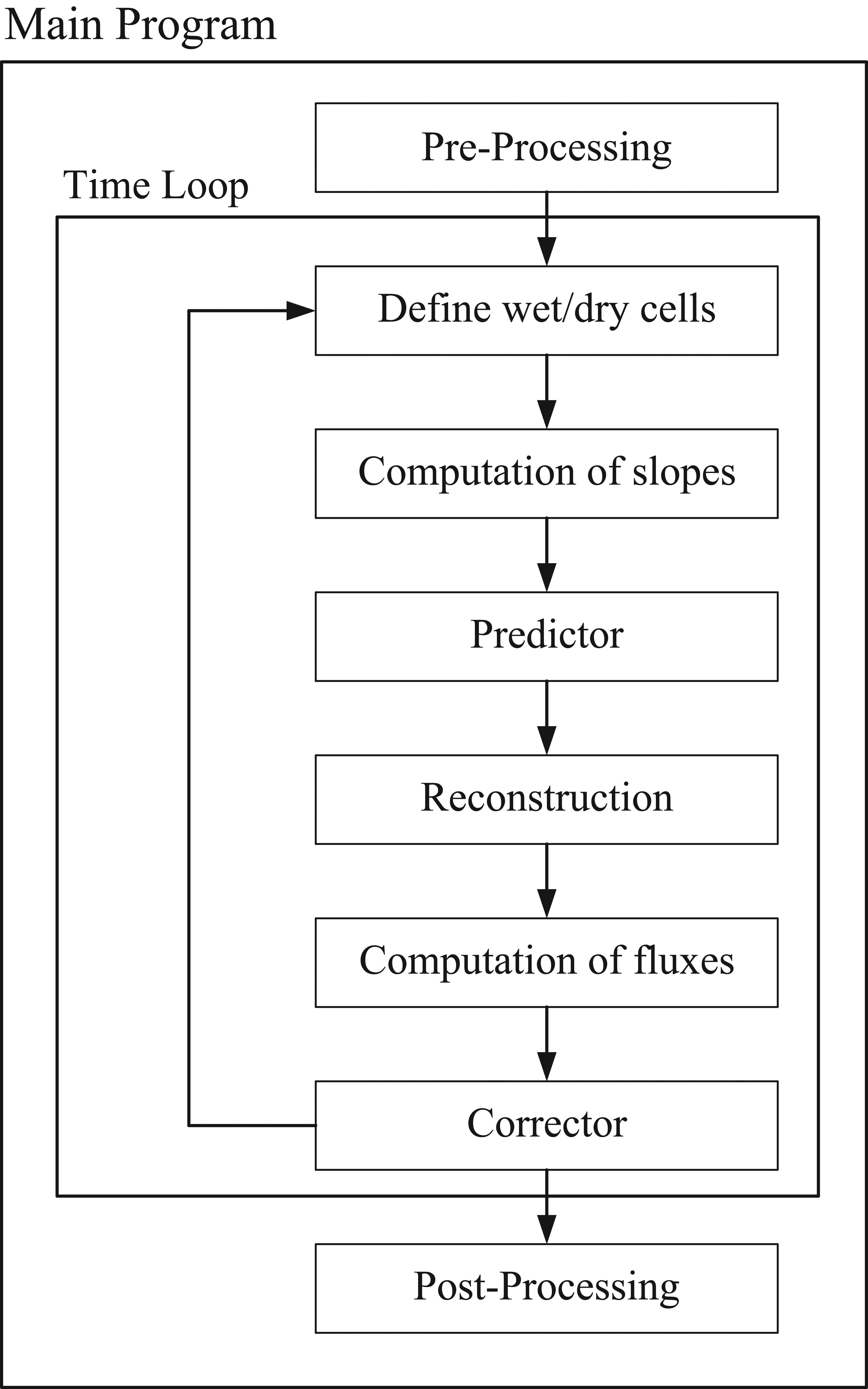
Algorithm flowchart.
Pre-processing
The mesh topology and model parameters are set in the pre-processing subroutine. The mesh topology includes three basic elements, that is, node, edge, and cell. A node has some information including coordinates, the bed elevation, cells around the node, and the weighted coefficients for interpolation. An edge has some information including left and right cells, start and end nodes, unit outward normal vector, and length. From the start node to the end node, a cell at the left side of the edge is defined as the left cell. The direction “left cell to right cell” is defined as the outward direction. A cell has some information including coordinates and bed elevation of centroid, area, Manning coefficient, three nodes, three edges, three adjacent cells, bed slopes in the
Wet or dry cell classification
To achieve a robust wetting and drying simulation while having in mind that cells’ data processing might be different whether it is wet or dry cell, the algorithm adopts a wet or dry cell classification to identify cells’ state. The horizontal free surface classification method proposed by Begnudelli and Sanders
17
is adopted in this article, that is, cells are classified as wet only when the water level is higher than the highest nodal bed elevation. It should be noted that the water level
Limited slope evaluation
Limited slopes of primitive variables
Predictor
The primitive variables
If the ith cell is classified as dry, then the predictor results are given by

If the ith cell is classified as wet, then the predictor results are given by


where the superscript
Reconstruction
The primitive variables

where the superscript Rec indicates the reconstructed value; and
Flux computation
First, at the midpoints of edges,
Corrector
The solution is advanced from
In the ith cell classified as wet, the conserved vector is first updated using numerical fluxes and bed slope estimation

where

and then the intermediate velocities are further updated using a semi-implicit scheme for friction4,8
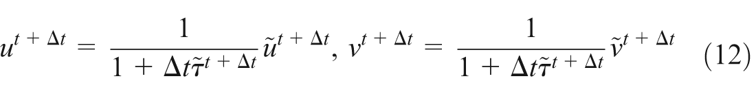
where
In the ith cell classified as dry, two different approaches might be adopted for updating. As for the first method proposed by Begnudelli and Sanders, 4 only the continuity equation is updated, whereas the velocity is set to zero. The second approach updates the continuity and momentum equations in dry cells and adopts the DFB (divergence form for bed slope source term) technique proposed by Valiani and Begnudelli 21 for bed slope estimation

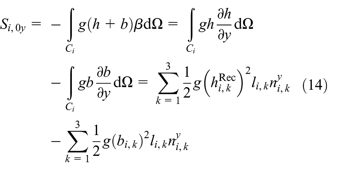
where
Methods selection for slope limiting and dry cell updating
In this section, we test two slope limiting approaches and two dry cell updating methods described above. The following notations are used for concision:
L1: slope limiting approach proposed by Barth and Jespersen 18 and limits at vertices;
L2: slope limiting approach proposed by Hubbard 19 and limits at edge midpoints;
U1: only the continuity equation is updated in dry cells, whereas the velocity is set to zero; 4
U2: the continuity and momentum equations are updated in dry cells, but the DFB technique is used for bed slope estimation.
Four different combinations, L1U1, L1U2, L2U1, and L2U2, are tested by modeling the following field-scale case of Paute River dam-break flood.
In 1993, the failure of a mountainside created a dam which blocked the flow of the Paute River. The dam subsequently breached causing a dam-break flood. This test case was used by Song et al. 8 to show the applicability of model to real case studies characterized by complex topography; however, oscillations are predicted by the proposed model. In this article, four combinations mentioned above are tested to assess these oscillations.
The model settings including topography, grids, boundary conditions, Manning roughness coefficient, and initial conditions are the same as those used by Song et al. 8 The coordinates of the six surveyed points are as follows: A (736,275 m, 9,686,020 m); B (739,144 m, 9,684,494 m); C (740,763 m, 9,683,922 m); D (744,446 m, 9,683,797 m); E (748,005 m, 9,686,389 m); and F (748,671 m, 9,690,875 m). We run the simulations until 6000 s after the start of dam-breaking. Figure 2(a)–(f) presents the simulated hydrographs at the surveyed points A–F. Results show that the effect of dry cell updating method on the simulated hydrographs is much more significant than that of slope limiting approach. Especially, upstream water release simulated using U2 (see results of L1U2 and L2U2) is faster than that simulated using U1 (see results of L1U1 and L2U1; Figure 2(a) and (b)), and the elapsed time until arrival of flood at the downstream surveyed points predicted using U2 is shorter than that predicted using U1 (Figure 2(d)–(f)). Since the velocity in dry cell is zero when using U1, while water moves in dry cell when using U2, so flood propagates faster when using U2, and then, the corresponding speeds of upstream water release and downstream flooding are faster. Besides, oscillations exist in the results predicted using L1U1, L2U1, and L2U2 (Figure 2(c) and (d)), whereas the results predicted using L1U2 is much smoother without remarkable oscillations (Figure 2(c)–(f)). So, the L1 and U2 are selected for modeling in this article. However, all simulations are run on a PC with a core 2 2.4-GHz processor, and the run time of the proposed algorithm with L1U2 was about 74 min, which is smaller than the simulation time.

Paute River dam-break flood: the computed hydrographs at surveyed points: (a) point A, (b) point B, (c) point C, (d) point D, (e) point E, and (f) point F.
Numerical results and discussions
Test 1: dam-break problem with a bottom step
The exact solution of ideal dam-break problem with a bed step was presented in the published literatures.22,23 In this test, a 25-m-long, 1-m-wide horizontal, frictionless, rectangular channel is used. The dam is located at 10 m from upstream end of the channel. The upstream bed elevation and water depth are 0 m and 1.461837 m, respectively, whereas the downstream bed elevation and water depth are 0.2 m and 0.308732 m, respectively. The initial flow velocity is set to zero. The problem domain was triangulated with 2500 elements. Numerical solutions for the water depth and flow velocity along the central line of the channel at 1 s after the dam removal are shown in Figure 3(a) and (b), respectively. Results show that the computed water depth and flow velocity match the exact solutions well. Comparing to the solutions of dam-break problem in a horizontal channel, 15 there are discontinuities in water depth and flow velocity at the dam site where the channel has a bed step.

Dam-break problem with a bed step: (a) comparison of water depth at t = 1 s and (b) comparison of flow velocity at t = 1 s.
Test 2: preservation of still water with wet or dry fronts
To verify the well-balanced property of the proposed algorithm, we consider a quiescent flow in a 1-m-long and 1-m-wide frictionless domain with a two-dimensional hump in this test. The domain is closed by solid walls. The bed elevation is specified as follows

The initial conditions are stationary states with a constant water level of 0.1 m, which should be exactly preserved by a well-balanced numerical scheme. The hump is partially submerged with wet or dry fronts. A simulation is carried out until t = 500 s, using a mesh of 2500 grids. The simulated water level and unit discharge along the line y = 0.5 m at t = 500 s are presented in Figure 4(a) and (b), respectively. The results show that during the simulation, the water level seems unperturbed, and the zero velocity is reproduced exactly, verifying the well-balanced property of the proposed algorithm.

Preservation of still water: (a) comparison of water level at t = 500 s and (b) comparison of unit discharge at t = 500 s.
Test 3: dam-break flow over two trapezoidal humps
Aureli et al. 24 performed dam-break experiment in a frictional channel with two humps. This test case has been employed for model testing as it simultaneously includes propagating bores and reflection waves, wetting and drying, surface curvatures, and steady-state equilibrium. 25 As shown in Figure 5, the channel is 7 m long and involves two trapezoidal humps (hump A and hump B). The dam is built along the central line on the top of hump A. Upstream of the dam, the initially stationary water level is set to 0.45 m, and the downstream area is initially dry. In addition, the upstream boundary is assumed to be close, while the downstream boundary is set to be transmissive.

Dam-break flow over two trapezoidal humps: side view channel layout.
The constant Manning roughness coefficient is set at 0.01 s/m1/3. 25 The upstream and lateral boundary is solid wall, whereas the downstream boundary is free outflow. The dam collapses instantaneously at t = 0. A simulation is carried out until t = 300 s. Figure 6(a) and (b) presents the simulated water level and unit discharge at t = 0, 1, 5, 10, and 300 s, respectively. The phenomena including bores propagation, wave interaction, movable wet or dry fronts, and surface curvatures are reasonably simulated (Figure 6(a)). Besides, the expected steady state is nearly reached at t = 300 s (Figure 6(b)). The results are very similar to that presented by Kesserwani and Liang. 25 The time evolution of water depth was recorded during 15 s after the dam removal at three spots located at x = 1.4, 2.25, and 4.5 m. The time evolution of velocity was also recorded at the gauge point located at x = 1.4 m. Figure 7(a)–(d) presents reasonably well comparisons between experimental data and numerical predictions, and the errors between the simulated results and the measured are presented in Figure 8 in which h_erros and u_erros represent the errors of depth and flow velocity, respectively. The elapsed time until arrival of flood is also accurately predicted by the proposed algorithm.
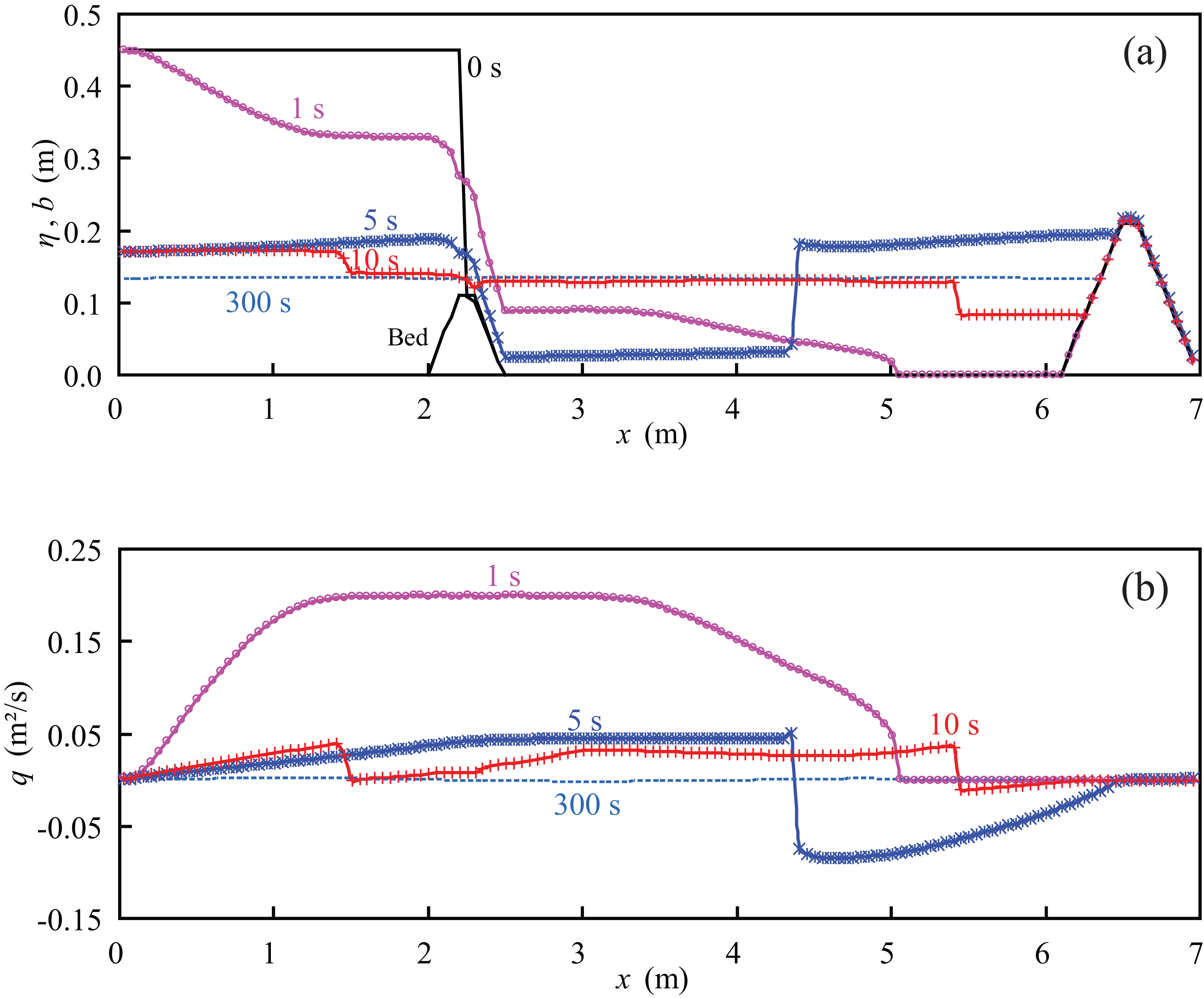
Dam-break flow over two trapezoidal humps: (a) the simulated water level at different output times and (b) the simulated unit discharge at different output times.

Dam-break flow over two trapezoidal humps: (a) the water depth at x = 1.4 m, (b) the water depth at x = 2.25 m, (c) the water depth at x = 4.5 m, and (d) the velocity at x = 1.4 m.

Dam-break flow over two trapezoidal humps: the errors between the simulated results and the measured.
Application: numerical simulation of dam-break flood over realistic topography
This section presents a practical application of realistic dam-break flood routine. Figure 9 shows the study domain and topography, from which we can see that the geometry is highly complex and the topography is very irregular. As the dam-breaking is a sudden event which always releases large amounts of water from reservoir, there is no available historical data related to branches and downstream sites, so the boundary of the computational domain should be chosen carefully, that is, the area should be large enough that floods do not flow to the boundary.
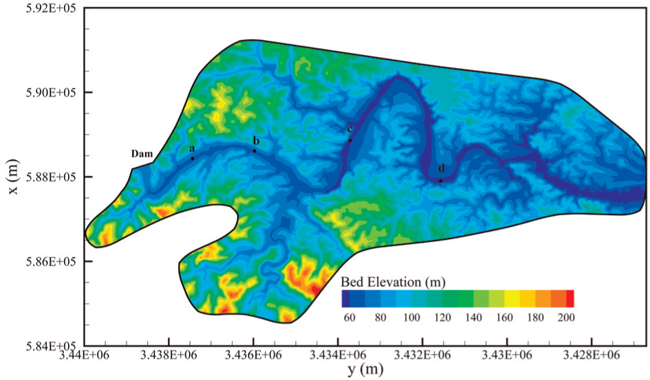
Computational domain and topography of the realistic dam-break problem.
Over 300,000 elements are used for domain triangulation. The minimum length of edges is 10.12 m, and the minimum area of grids is 70.16 m2. Four study points are plotted in Figure 9: a (588,433 m, 3,437,439 m), b (588,612 m, 3,435,975 m), c (588,860 m, 3,433,713 m), and d (587,906 m, 3,431,572 m). The inflow of the predefined discharge at the dam site is presented in Figure 10.

Inflow condition of the predefined discharge at the dam site.
A uniform value of 0.03 s/m1/3 of Manning roughness coefficient is used in the simulation. A dry bed condition is adopted as the initial condition to test the model stability for wetting and drying. The computation was run until the time t = 75 min. Figure 11(a)–(h) presents the filled contour plot of the simulated water depth at time t = 5, 10, 15, 25, 35, 45, 65, and 75 min. As shown in Figure 11, the flood wave fronts move very fast, especially in the first 35 min. Due to the decrease in the inflow discharge and the storage effect of river, the flood wave fronts move slower after t = 35 min. Results also show the well-simulated flooding and recession process. Figures 12 and 13 present the maximum flood depth and the flood arrival time in 75 min after dam-break, respectively. The flood risk information is very important for disaster prevention and reduction.
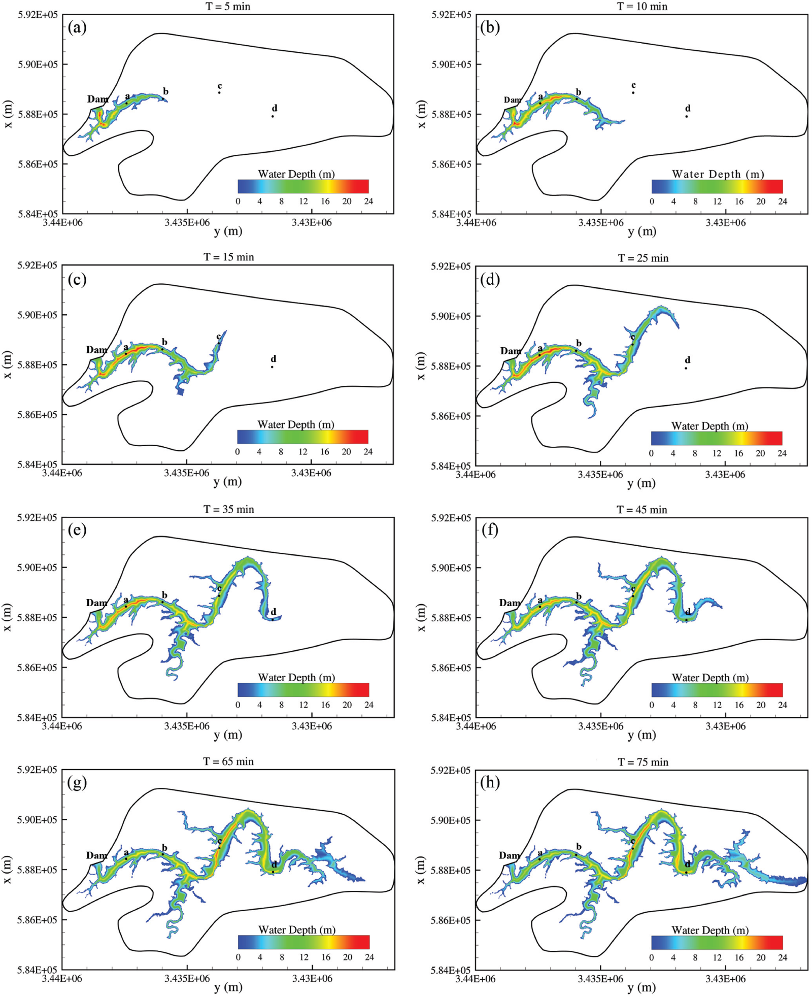
Filled contour plot of simulated water depth at time (a) t = 5 min, (b) t = 10 min, (c) t = 15 min, (d) t = 25 min, (e) t = 35 min, (f) t = 45 min, (g) t = 65 min, and (h) t = 75 min.

Maximum flood depth in 75 min after dam-break.

Flood arrival time in 75 min after dam-break.
To test the influence of Manning roughness on numerical results, the uniform Manning coefficient is set at 0.025, 0.04, and 0.05 s/m1/3. Figure 14 presents the water level comparisons at four study points. Results show that during the beginning period of the flooding, water levels at four study points increase quickly, and the increasing speeds at points a and b are relatively greater than those of points c and d. This could be due to the storage and delay effect of the river and floodplain. Furthermore, as the Manning roughness coefficient increases, the move speed of flood front decreases, but the highest water level increases. Table 1 shows the statistical values of flood arrival time and maximum water level at four study points. Since the flood peak does not arrive at point d at time t = 75 min (see Figure 11(h)) while the flood front has arrived at the downstream boundary, the highest water level at point d could not be provided by this simulation. More simulations should be done to evaluate the influence of downstream boundary on the highest water level at point d. If the influence is obvious, then the computational area should be enlarged.

Water-level comparisons at four study points: (a) point a, (b) point b, (c) point c, and (d) point d.
Flood arrival time and maximum water level at study points.

Conclusion
An improved hydrodynamic model based on a new formulation of the two-dimensional shallow water equations and Godunov-type finite volume scheme is developed in this article for simulating flood wave propagation over arbitrary topography. The model uses HLLC approximate Riemann solver to compute fluxes and adopts Hancock’s predictor–corrector scheme for efficient time stepping. Two slope limiting approaches (L1 and L2) and two dry cell updating methods (U1 and U2) are tested through a field-scale case of Paute River dam-break flood. Results of the tests mentioned above show that the effect of dry cell updating method on numerical prediction is much more significant than that of slope limiting approach. In case of setting a zero velocity in dry cell (U1), the speed of flood propagation would be reduced. All three following combinations, L1U1, L2U1, and L2U2, produce oscillations, whereas only L1U2 predicts smooth results without remarkable numerical oscillation. So, L1 is chosen for slope limiting, and U2 is adopted for dry cell updating in this article. Besides, the run time of 74 min for the Paute River dam-break flood simulation shows the efficiency of the proposed algorithm.
Based on the case study about the numerical oscillation, a new hybrid method is suggested for bed slope terms approximation, that is, the bed slope terms in wetted cells are exactly discretized based on central values, whereas the DFB approximation approach is adopted for partially wetted cells. As the basis for cell updating, this new hybrid method provides an alternative way that precisely preserves the well-balanced property of the algorithm for simulations involving wet or dry fronts.
Several benchmark test cases including ideal dam-break problem with a bed step, quiescent flow with wet or dry fronts, and laboratory experiments of dam-break are used for model validation. The reasonable good agreement between numerical and reference results demonstrates the effectiveness and robustness of the proposed algorithm. Furthermore, the proposed model is used for a practical application of realistic dam-break flood routine. Numerical results show that the model can account for dam-break floods with respect to its effectiveness and robustness and thus has bright application prospects.
Footnotes
Academic Editor: Cheng-Xian Lin
Declaration of conflicting interests
The author(s) declared no potential conflicts of interest with respect to the research, authorship, and/or publication of this article.
Funding
The author(s) disclosed receipt of the following financial support for the research, authorship, and/or publication of this article: This work was financially supported by the National Natural Science Foundation of China (nos 51279013, 11202037), the PhD Start-up Fund of Natural Science Foundation of Guangdong Province, China (no. 2014A030310283), the Open Research Foundation of PRHRI (no. 2013KJ01), the National Public Research Institutes for Basic R&D Operating Expenses Special Project (no. CKSF2013024/SL), and National Science & Technology Pillar Program during the 12th Five-Year Plan Period (no. 2012BAK10B04).