Sage Journals: Discover world-class research

Abstract

It is very important to study fluid–structure interaction of vehicles which move in strong crosswind environment. For solving a fluid–structure interaction problem, the effect of the deformation and vibration of the elastic body on the flow field should be considered. However, the reaction of the vibrating flow field on the vehicle body should be computed. A kind of coach model is selected for solving the fluid–structure coupling problem. We have considered the interaction of the deformation of vehicle suspension and the displacement of sprung mass and the flow field around the coach model using a numerical simulation. The coupling method is partitioned but loosely coupled with the Fluent software to describe the flow field and the ANSYS software to describe the reaction of the structure. The numerical results are in good agreement with the experimental data.

Keywords

Fluid–structure interaction bluff body numerical simulation wind tunnel test

Introduction

The stability control is directly related to the safety of a vehicle, which is mainly based on the forces and moments due to flow field around vehicle body and the response of vehicle body, especially in the high speeds. The stability analysis has been regarded as a very important issue in the vehicle aerodynamic researches. In crosswind, the deformation of suspension will cause notable deviations in the aerodynamic lateral force and lift force (especially for coaches with high aspect ratio of cross section), and therefore, the driving safety is deteriorated.

The significance of stability control and the complexity of the crosswind forcing mechanisms have led to a considerable amount of research work, either experimental or numerical. The aerodynamic forces acting on a moving vehicle passing through the wake of a bridge tower under crosswind by a numerical–experimental methodology were studied by Rocchi et al.¹ Tsubokura et al.² studied the unsteady aerodynamic response of a road vehicle in transient crosswinds by a computational fluid dynamics (CFD) method with large-eddy simulation (LES) turbulence modeling. Suzuki et al.³ considered three kinds of wind tunnel tests to evaluate the aerodynamic characteristics of typical configurations of infrastructures such as bridges and embankments.

The crosswind causes deformation of vehicle. Although some studies on such phenomenon have been carried out by several authors^4,5 with system simulation method, one cannot see enough quantified researches on the rolling traits of sprung mass. The existing analysis method is limited in the scope of system dynamics; the research results have no interpretation from the prospect of fluid mechanism. With the development of computer performance and simulation technology, the fluid–structure interaction (FSI) analysis in the crosswind is necessary and feasible.

In the application of FSI, we can consider loose coupling and strong coupling between the fluid and the structure. For loose coupling, typically the arbitrary Lagrangian–Eulerian (ALE) method is used where the flow equations are discretized on a moving grid that follows the motion of the structure. With loose coupling FSI method, a time-accurate computational analysis of vertical tail buffeting of full F/A-18 aircraft was conducted by Sheta and Huttsell.⁶ For biomedical and biological applications, typical compliant structures such as vessels or membranes in strongly coupling problems have been studied by Lemmon and Yoganathan.⁷

Many technological problems in engineering can be described using loosely coupling methods for FSI, such as industrial chimney,⁸ turbomachinery,⁹ bridges,¹⁰ and so on. This study focuses on the case of FSI problems characterized by bluff body considering suspension system, when the local deformation is negligible compared to the displacement. As solid, the structure of body and suspension can be accurately modeled with a finite element formulation. For vehicles moving near ground, the air is considered as an incompressible fluid. Since the meshes of structure and fluid domain on the coupling interface are not exactly matched in the simulation, interpolation is required when parameters are transferred to each other on both sides of the interface to study the FSI problem.

This article is organized as follows: in section “Mechanical model of vehicle structure,” the mechanical model of vehicle structure is briefly explained. Section “Fluid model” describes the fluid model, section “Fluid–structure coupling” describes the fluid–structure coupling method, and section “Coupling computational method validation” describes the coupling computational method validation by simple model experiment. Section “Coach model under crosswind action” presents the calculation result of a coach model and section “Conclusion” concludes by summarizing the main aspects of the work.

Mechanical model of vehicle structure

The vehicle structure was modeled by the entity element in ANSYS (Figure 1). The computational restriction was the fixed connection constraint between the wheels and ground; other surfaces were defined as fluid–solid interface. The related mechanical parameters of the air spring were the elastic modulus E = 27.8 MPa, damping factor β = 0.15, and density ρ = 1000 kg/m³.

Figure 1.

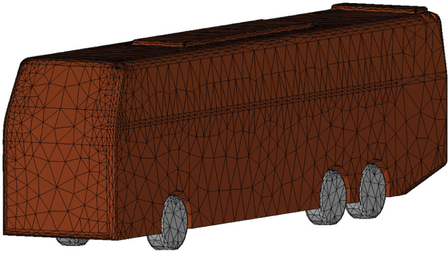
Element of coach model structure.

According to the characteristic of air spring suspension system, the 6-degree-of-freedom space movement model of coach was established and is shown in Figure 2. The dynamic matrix reaction between external forces and general displacements can be described by the following equation

M \overset{\cdot\cdot}{x} + k \overset{\cdot}{x} + cx = F (t)

(1)

where M is the mass matrix, k is the stiffness matrix, c is the damping matrix, and F(t) is the load imposed by the fluid, which includes surface pressure and shear stress. For the membrane structure,¹¹ the shearing strength cannot be neglected normally; but for coach structures, the effect of shear strength imposed by the fluid is low, and the structure is not sensitive to the shearing strength action. The dynamic reaction of the coach body is described by the body’s displacement x, the speed $\overset{\cdot}{x}$ , and the acceleration $\overset{\cdot\cdot}{x}$ . Especially, the fluid damping is included in the right term of equation (1); it is not in the damp matrix c.

Figure 2.

Six-degree-of-freedom model of system dynamics.

Fluid model

The Reynolds-averaged Navier–Stokes (RANS) model has acceptable accuracy in the vehicle engineering applications. For incompressible fluid, the momentum equations can be expressed as

\frac{\partial \bar{u_{i}}}{\partial t} + \bar{u_{j}} \frac{\partial \bar{u_{i}}}{\partial x_{j}} = - \frac{1}{ρ} \frac{\partial \bar{p}}{\partial x_{i}} + v \frac{\partial^{2} \bar{u_{i}}}{\partial x_{j} \partial x_{j}} - \frac{\partial \bar{{u'}_{i} {u'}_{j}}}{\partial x_{j}}

(2)

For solving these equations by a numerical method, the unknown Reynolds stresses term must be modeled. For modeling the Reynolds stresses, we have used standard k–ε turbulence model. Based on Boussinesq assumption,¹² the relationship between Reynolds stresses and mean quantities of the flow field is given by

- ρ \bar{u'_{i} u'_{j}} = μ_{t} (\frac{\partial \bar{u_{i}}}{\partial x_{j}} + \frac{\partial \bar{u_{j}}}{\partial x_{j}}) - \frac{2}{3} (ρ k + μ_{t} \frac{\partial \bar{u_{i}}}{\partial x_{i}}) δ_{ij}

(3)

where $μ_{t}$ is turbulence dynamic viscosity, k is kinetic energy, and $δ_{ij}$ is Kronecker delta.

For determining $μ_{t}$ , according to semi-empirical assumption, the turbulence model is closed by introducing two equations of kinetic energy k and diffusion rate ε. The control equations of k and ε are as follows

\frac{\partial (ρ k)}{\partial t} + \frac{\partial (ρ k \bar{u_{i}})}{\partial x_{i}} = \frac{\partial}{\partial x_{j}} [(μ + \frac{μ_{t}}{σ_{k}}) \frac{\partial k}{\partial x_{j}}] + G_{k} - ρ ε

(4)

\begin{matrix} \frac{\partial (ρ ε)}{\partial t} + \frac{\partial (ρ ε \bar{u_{i}})}{\partial x_{i}} \\ = \frac{\partial}{\partial x_{j}} [(μ + \frac{μ_{t}}{σ_{ε}}) \frac{\partial ε}{\partial x_{j}}] + C_{1 ε} \frac{ε}{k} G_{k} - C_{2 ε} ρ \frac{ε^{2}}{k} \end{matrix}

(5)

where G_k represents the turbulent kinetic energy created by the average velocity grads, $C_{1 ε} = 1.44$ , $C_{2 ε} = 1.92$ , $σ_{k} = 1.0$ , and $σ_{ε} = 1.3$ , determined by the classical experiments.

In this article, due to the importance of wall function in the computation, a two-layer-based, nonequilibrium wall function¹³ was adopted to describe the structure of boundary layer. Different from the standard wall function, the log-law for mean velocity sensitized to pressure gradients is

\frac{\tilde{U} C_{μ}^{1 / 4} k^{1 / 2}}{τ_{w} / ρ} = \frac{1}{k} \ln (E \frac{ρ C_{μ}^{1 / 4} k^{1 / 2} y}{μ})

(6)

where

\tilde{U} = U - \frac{1}{2} \frac{dp}{dx} [\frac{y_{v}}{ρ k \sqrt{k}} \ln (\frac{y}{y_{v}}) + \frac{y - y_{v}}{ρ k \sqrt{k}} + \frac{y_{v}^{2}}{μ}]

(7)

The physical viscous sublayer thickness $y_{v}$ is computed from

y_{v} \equiv \frac{μ y_{v}^{*}}{ρ C_{μ}^{1 / 4} k_{P}^{1 / 2}}

(8)

where $y_{v}^{*} = 11.225$ .

The nonequilibrium wall functions are more accurate for describing the wake behind vehicles because the mean flow and turbulence are subjected to severe pressure gradients and change rapidly.

Fluid–structure coupling

Generally, two methods are used for fluid–structure coupling analysis: strongly coupling and loosely coupling. For strongly coupling method, the whole set of equations of fluid and structure need to be built in the same form and solved synchronously. Furthermore, the consistency of grid nodes on the interface surfaces must be guaranteed. So, this method is usually adopted in the theoretical problems with geometric simplification.¹⁴

Compared with strongly coupling method, the advantage of loosely coupling method is that CFD code and computational structural dynamics (CSD) code can be fully developed independent of the predominance of each other. Based on data exchanging platform between the structure field and the flow field, loosely coupling method solves the CFD and CSD equations and, in turn, in each time step, it solves the aerodynamic force by CFD code and the dynamic parameters of the structure reaction by CSD code.

Current work focuses on a bluff body, in particular, a rectangular cross-sectional body, with a clear predominance of the shape resistance over the friction resistance. The flow field around the body is characterized by large Reynolds numbers and flow separation around the body cross section. It is concluded that loosely coupling method¹⁵ is very efficient for solving such FSI problem. In the coupling scheme, the structural solution is integrated in the fractional step procedure, and the ALE¹⁶ formulation is used to take into account the deformation and re-meshing of the fluid mesh.

The time step iteration algorithm of loosely coupling method for solving the fluid–structure problem is shown in Figure 3. The vertical direction represents the progress of the time step, the horizontal direction represents the current status, and the arrow head means the calculation procedure.¹⁷ According to the procedure depicted in Figure 3, the calculation started from the CFD model. After one time step Δt, the wind load P obtained will return to the CSD model for transient analysis. After another time step Δt, the moving speed of the structure obtained from CSD will return to the CFD model. Due to the deformation of the CFD mesh, the new solution of the flow field will be obtained. This procedure is repeated until the designed convergence value is achieved.

Figure 3.

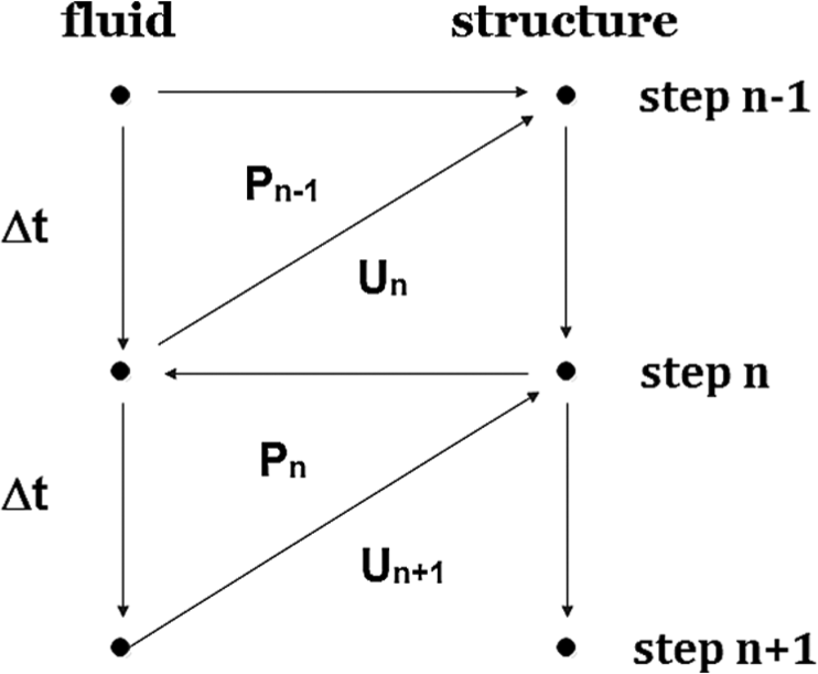
Time step iteration algorithm.

For FSI problem simulation, the movement of mesh is inevitable. Generally, the flow dynamic transport equation of viscous fluid described by finite volume is given as

\begin{matrix} \frac{d}{dt} \int_{v} ρ ϕ dv + \int_{v} [ρ (u - u_{g}) ϕ - Γ_{ϕ} grad ϕ] \\ \times ndS = \int_{v} S_{ϕ} dV \end{matrix}

(9)

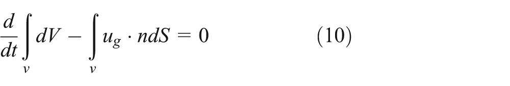
where for the continuity equation, $ϕ = 1$ ; for the momentum equation, $ϕ = (u, v, w)$ ; and for the k–ε turbulence model, $ϕ = (k, ε)$ . The diffusion coefficient $Γ_{ϕ}$ and source term $S_{ϕ}$ are selected by the value of $ϕ$ .

In the case of transient moving mesh, the value of the transport speed is equal to the residual value of Euler speed or absolute speed minus the moving mesh speed u_g. In order to ensure the conservation of mass, the following equation must be satisfied for each control volume

\frac{d}{dt} \int_{v} dV - \int_{v} u_{g} \cdot ndS = 0

(10)

ALE method introduces the conception of “mesh flux” across the control surfaces to replace the integral term of the moving mesh speed so as to avoid direct calculation of the moving mesh speed. The movement of the control surface during the iteration process is the source of “mesh flux.” So, in discrete form, the convective term including the moving mesh speed in the transport equation could be written as

\int_{v} ρ ϕ u_{g} \cdot ndS \approx \sum ρ_{c} ϕ_{c} \frac{δ V_{c}}{Δ t}

(11)

Based on the flux passing through the control volume caused by fluid motion minus “mesh flux,” every transport equation is solved. The moving mesh speed is not required as a known parameter of the flow region but given explicitly at the moving nonpenetrating wall. Furthermore, the boundary conditions are available as in the case of normal CFD simulation.

Coupling computational method validation

A 1/4-scale Ahmed body¹⁸ with a backward angle of 25° was taken for validation, whose length was 260 mm. For researching the FSI problem, special spring system of Ahmed body was designed, which consisted of spring, packing, and copper sleeve with which the system was fixed on the ground, as shown in Figure 4.

Figure 4.

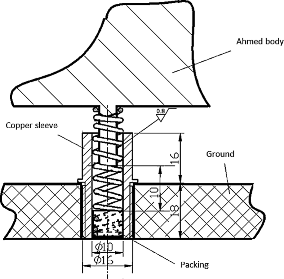
Cross section of spring system.

The 4 degrees of freedom of the dynamic model was adopted to simulate the dynamical behavior of improved Ahmed body that is supported by four springs (elastic coefficient 3921 N/m) with total weight of 705 g. The experiment was carried out in a 1/15-scale open-jet wind tunnel, as shown in Figure 5. Relative to the flow direction, the yaw angle was 90°, and the inlet velocity of nozzle was selected as 20, 25, 30, 35, and 40 m/s.

Figure 5.

Installation location of Ahmed body in wind tunnel.

In numerical study, the calculation domain was divided into fluid zone and structure zone, and all of the zones were discretized with tetrahedron meshes. For fluid simulation, a typical surface mesh element had a size of 10 mm, and the smallest surface element had a size of around 1 mm surrounding support poles of model body. The surfaces of the virtual wind tunnel were discretized also with triangle mesh elements about 200 mm. There were about 2,000,000 cells in the fluid zone and about 40,000 elements in the structure zone. The surface mesh on the interface which belongs to the fluid zone and the structure zone is shown in Figure 6.

Figure 6.

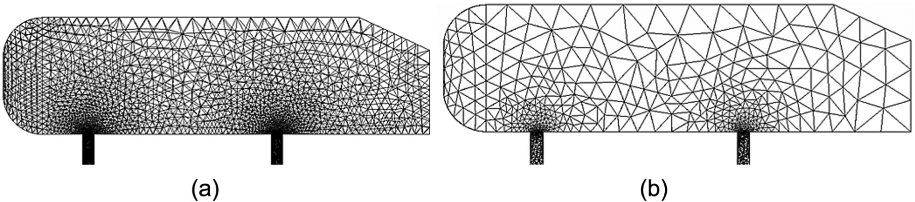
Surface mesh on the interface of Ahmed body: (a) fluid and (b) structure.

Finite volume method (FVM) and finite element method (FEM) were adopted to calculate the parameters of the fluid zone and the structure zone, respectively. The k–ε model and impermeable boundary condition were used for flow field simulation. A linear model was used for structure reaction simulation. The surface displacement of the structure and the pressure of the flow field on the interaction face were transferred to each other by profile preserving interpolation and conservative interpolation¹⁹ with the relaxation factor set as 0.8. FSI coupling process began from fluid zone. In the studied cases, the wall y+ values were mainly in the range of 30–300, and wall functions were indeed valid.

Because ALE method was adopted, dynamic mesh option was activated for numerical simulation. On account of topological homeomorphism and moderate deformation, only spring-based smoothing model²⁰ was used in the dynamic mesh processing. For better mesh quality, elasticity coefficient and boundary node relaxation factor were 0.6 and 0.5, respectively. The displacement of improved Ahmed body measured by wind tunnel test is shown in Figure 7, and the displacement and the deformation of mesh simulated by numerical method are shown in Figure 8. The comparison of deformation angle that is shown in Figure 9 illustrates the consistency of test data and simulation results.

Figure 7.

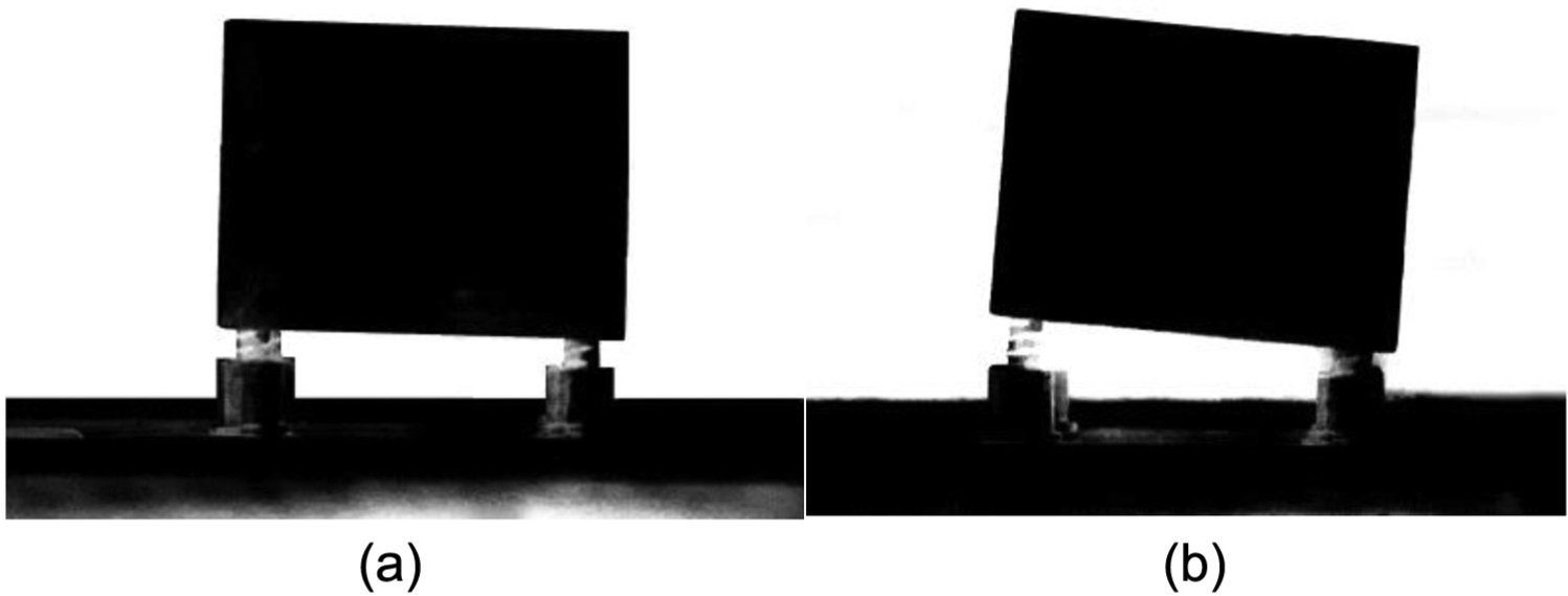
Displacement of Ahmed body measured by wind tunnel test: (a) 20 and (b) 40 m/s.

Figure 8.

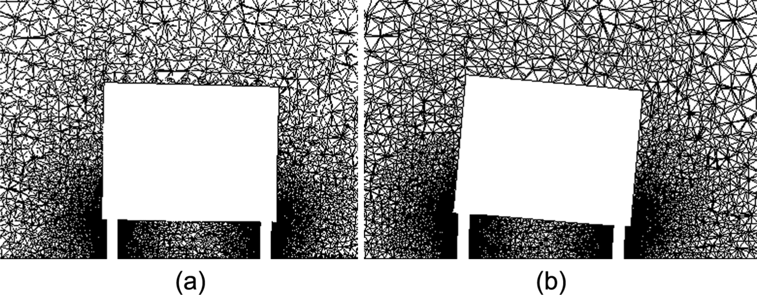
Displacement of Ahmed body simulated by numerical method: (a) 20 and (b) 40 m/s.

Figure 9.

Deformation angle of Ahmed body.

Generally, the simulation results of body deformation were greater than test data because of the inevitable surface contact friction of sleeve and special spring system. When the wind speed was 20 m/s, there was small deviation between simulation results and test data due to little friction with small deformation of special spring system. As the wind speed increased gradually, the deformation and friction increased simultaneously. Because the wind load overcame the friction resistance when the wind speed was 40 m/s, the simulation results agreed with the test data well again (error = 2.6%).

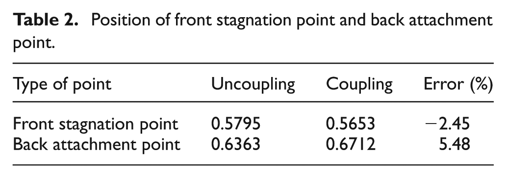
The difference in vortex topological structure shown in Figure 10 illustrates that the structure of attached vortex above the Ahmed body is more complicated when FSI is considered. Because of the obvious separate bubble on the top of Ahmed body, the lower pressure causes an increase in aerodynamic lift force on Ahmed body. Table 1 shows aerodynamic force components, and Table 2 shows the relative position of front stagnation point and back attachment point.

Figure 10.

Vortex topological structure around Ahmed body: (a) uncoupling simulation and (b) coupling simulation.

Table 1.

Aerodynamic force components.

Components	Uncoupling (N)	Coupling (N)	Error (%)
Lateral force	11.96	12.38	3.51
Lift force	1.439	3.374	134.47

Table 2.

Position of front stagnation point and back attachment point.

Type of point	Uncoupling	Coupling	Error (%)
Front stagnation point	0.5795	0.5653	−2.45
Back attachment point	0.6363	0.6712	5.48

Based on the data of wind tunnel test, the numerical method of FSI problem simulation was validated. Furthermore, the difference between simulation results of uncoupling and coupling method was compared and analyzed.

Coach model under crosswind action

The resulting coach model has an overall length of 13.67 m, width of 2.55 m, and height of 3.96 m and a frontal area of 10.10 m². The computational domain was set to be 96.00 m in length, 54.00 m in width, and 20.00 m in height.

The structure zone and fluid zone were discretized with unstructured tetrahedron mesh. For fluid simulation, a typical surface mesh element had a size of 250 mm, and the smallest surface element had a size of around 20 mm surrounding the details and wheels of coach model body. The surfaces of the virtual wind tunnel were discretized also with triangle mesh elements, about 500 mm. There were about 8,000,000 elements in fluid zone and 80,000 elements in structure zone. Figure 11 shows the surface mesh on the interface which belongs to fluid zone. Cells of prismatic layers were created just off the vehicle surfaces (including the underbody) in order to better resolve the boundary layers over the coach surfaces. In the cases studied, the wall y+ values were mainly in the range of 30–300, and wall functions were indeed valid.

Figure 11.

Surface mesh on the interface of fluid zone.

Spring-based smoothing model and re-meshing method were used in the dynamic mesh processing. For better mesh quality, elasticity coefficient and boundary node relaxation factor were 0.6 and 0.5, respectively, and 50 iterations were set for data transfer of interface surfaces.

The parameters on the interaction surfaces of different zones were transferred to each other by profile preserving interpolation and conservative interpolation with the relaxation factor set as 0.8. The time step was set to 0.01 s, and the total simulation time was 5 s. In each time step, 30 iterations were set for solving flow field, and 10 iterations were set for FSI processing.

The boundary conditions for the computation were set as follows: in order to simulate the behavior of crosswind, two kinds of inlet surfaces were used. For the inlet surface in front of coach model head without crosswind, the incoming velocity was set to U (X direction velocity) = 30 m/s, V (Y direction velocity) = W (Z direction velocity) = 0 m/s, turbulence level of Tu = 1%. For the inlet surface next to the left side of coach model with crosswind, the incoming velocity was set to V = 4t m/s, where t is crosswind lasting time from 0 to 5 s, U = W = 0 m/s, turbulence level of Tu = 1%. At the exit of computational domain, the pressure outflow condition was specified. Inviscid moving wall condition was applied at the floor. Symmetry condition was selected at the top of the virtual wind tunnel. At the coach model surfaces, velocity of flow was set to 0. It means that the simulation solves the FSI problem of a coach moving in gust of crosswind which lasts for 5 s.

The acceleration, velocity, and displacement time history of sampling point on the coach model body are plotted in Figure 12. Figure 13 shows the displacement of coach body at the end of simulation. The absolute value of maximum displacement is 0.117 m on the top of coach model.

Figure 12.

Acceleration, velocity, and displacement of sampling point.

Figure 13.

Deformation of coach model.

With uncoupling method and coupling method simulation, the calculation results of drag force, lift force, and lateral force on the coach model body are plotted in Figure 14. For drag force and lift force, besides the same increment trend, the value of coupling method simulation results is greater than uncoupling method simulation results under stronger crosswind. For lateral force, the results of coupling method simulation are almost the same as that of uncoupling method simulation. Table 3 shows aerodynamic force components at the end of simulation. The pressure difference of coach model simulated by uncoupling method and coupling method is shown in Figure 15. Because of the lower pressure on the top of coach model caused by separate bubble and higher pressure under the bottom of coach model caused by lower velocity, there is a substantial discrepancy between the lift force and the pitching moment calculated by uncoupling method and coupling method, respectively.

Figure 14.

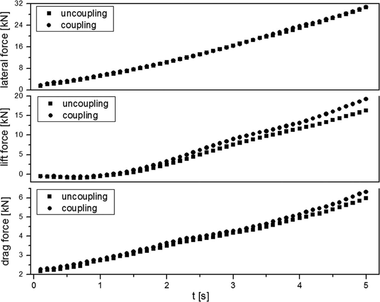
Drag force, lift force, and lateral force on coach model body.

Table 3.

Aerodynamic force components of coach model.

Components	Uncoupling, (N)/(N × m)	Coupling, (N)/(N × m)	Error (%)
Drag force	5847.9	6207.4	6.15
Lift force	16288.4	19183.4	17.77
Lateral force	30627.2	30722.2	0.31
Rolling moment	51196.1	51567.6	0.73
Pitching moment	16197.9	21124.2	30.41
Yawing moment	55705.8	56078.5	0.67

Figure 15.

Pressure difference of coach model.

When the velocity of crosswind was 10 m/s (t = 2.5 s), the deformation of coach model was too small to show FSI phenomenon, and the aerodynamic forces were roughly unchanged. But when the velocity of crosswind was greater than 10 m/s (t > 2.5 s), the FSI phenomenon was increasingly necessary to be solved with the increase in crosswind speed, as shown in Figure 14.

Figure 16 shows the deformation velocity of mesh in fluid zone including 25 frames (one frame per 2 s). Because of the control technology of boundary layer mesh and reasonable parameter setting, the velocity uniformity of boundary layer mesh and the topological homeomorphism of most mesh in fluid zone were guaranteed. It is seen from Figure 16 that deformation of mesh decreased and vanished when the location was gradually away from the coach model surface.

Figure 16.

Deformation velocity of mesh in fluid zone.

In this study, the requirement of computational resource including hardware and CPU time for coupling method is almost one order of magnitude higher than that for uncoupling method. Furthermore, the coupling method is less robust than uncoupling method.

Conclusion

A wind tunnel experiment for investigating FSI problem of simplified vehicle body (Ahmed body) has been developed. Despite its simplicity, the experiment can successfully capture the basic FSI physical behavior of bluff body under crosswind. The experiment data and snapshots of flow field visualization were obtained for validating the numerical method of FSI simulation.

The loosely coupling method based on the MFX-ANSYS or Fluent coupling platform can effectively calculate the fluid–structure coupling characteristics of the bluff body with suspension system. It is critical to define the coupling surface and determine the coupling time step. The coupling platform is between the software ANSYS and Fluent, which can exchange the calculated pressure in the flow field with the calculated displacement in the structure field.

When FSI is considered, stronger aerodynamic force on vehicle body and deformation of vehicle structure mean higher overturning risk of the vehicle due to directly blowing and driver’s mistakes because of misjudgments and psychological effect. All these results bring new possibilities and advances in the field of safety assessment and control stability simulation for vehicles under crosswind. The style of vehicle prototype, the performance parameter of suspension system, and the effectiveness of active and passive control devices for the suppression of vibrations of vehicles body can be estimated in early design stages.

Footnotes

Academic Editor: Elsa de Sá Caetano

Declaration of conflicting interests

The authors declare that there is no conflict of interest.

Funding

This work was financially supported by National Key Basic Research and Development Program (973) (2011CB711203).

References

Rocchi

Rosa

Sabbioni

. A numerical–experimental methodology for simulating the aerodynamic forces acting on a moving vehicle passing through the wake of a bridge tower under crosswind. J Wind Eng Ind Aerod 2012; 104–106: 256–265.

Tsubokura

Nakashima

Kitayama

. Large eddy simulation on the unsteady aerodynamic response of a road vehicle in transient crosswinds. Int J Heat Fluid Flow 2010; 31: 1075–1086.

Suzuki

Tanemoto

Maeda

. Aerodynamic characteristics of train/vehicles under crosswinds. J Wind Eng Ind Aerod 2003; 104–106: 256–265.

Wang

Luo

. Study on automobile cross-wind stability in consideration of pressure center’s shift. J Hunan Univ 2005; 32: 70–73.

Hai

Wang

. Research on the effect of crosswinds on the stability of high speed vehicles. J Hunan Univ 2006; 33: 40–43.

Sheta

Huttsell

. Characteristics of F/A-18 vertical tail buffeting. J Fluid Struct 2003; 17: 461–477.

Lemmon

Yoganathan

. Three-dimensional computational model of left heart diastolic function with fluid–structure interaction. J Biomech Eng Trans ASME 2000; 122: 109–117.

Belver

Iban

Martin

. Coupling between structural and fluid dynamic problems applied to vortex shedding in a 90 m steel chimney. J Wind Eng Ind Aerod 2012; 100: 300–307.

Carstens

Kemme

Stefan Schmitt

. Coupled simulation of flow–structure interaction in turbomachinery. Aerosp Sci Technol 2003; 7: 298–306.

10.

Braun

Awruch

. Finite element simulation of the wind action over bridge sectional models: application to the Guamá River Bridge (Pará State, Brazil). Finite Elem Anal Des 2008; 44: 105–122.

11.

Nakata

Liu

. A fluid–structure interaction model of insect flight with flexible wings. J Comput Phys 2012; 231: 1822–1847.

12.

Hinze

. Turbulence. New York: McGraw-Hill, 1975.

13.

Kim

Choudhury

. A near-wall treatment using wall functions sensitized to pressure gradient. In: ASME FED vol. 217, Separated and complex flow, 1995, pp.273–280. ASME.

14.

Yang

Stern

. A simple and efficient direct forcing immersed boundary framework for fluid–structure interactions. J Comput Phys 2012; 231: 5029–5061.

15.

Dadvand

Rossi

Onate

. An object-oriented environment for developing finite element codes for multi-disciplinary applications. Arch Comput Meth E 2010; 17: 253–297.

16.

Hirt

Amsden

Cook

. An arbitrary Lagrangian–Eulerian computing method for all flow speeds. J Comput Phys 1974; 14: 76–85.

17.

Mao

Yang

. Numerical simulation of the pneumatic elasticity for the blade of a big axial-flow fan. Eng Fail Anal 2011; 18: 1037–1048.

18.

Ahmed

Ramm

Faltin

. Some salient features of the time-averaged ground vehicle wake. SAE technical paper 840300, 1984.

19.

Dukowicz

Kodis

. Accurate conservative remapping (rezoning) for arbitrary Lagrangian–Eulerian computations. J Comput Phys 1987; 8: 305–321.

20.

Degand

Farhat

. A three-dimensional torsional spring analogy method for unstructured dynamic meshes. Comput Struct 2002; 80: 305–316.