
Abstract
The automotive frames that can be created consciously with three-dimensional freehand strokes are quite important and useful in the early stage of automotive styling. However, all the strokes are drawn on the screen in two-dimensional. This study focuses on the creation of three-dimensional freehand strokes by applying the interpolation algorithm in two orthogonal planes, the projection algorithm and the resultant matrix algorithm. The fitting algorithms of strokes have been developed as the bridges between the traditional two-dimensional sketching and three-dimensional digital modeling. The stylists could use the digital tablet and pen to sketch the frames or outlines of a vehicle in three-dimensional space and then those could be used for establishing the automotive surfaces in any engineering software.
Introduction
Freehand sketching used by automotive stylists is a traditional way to express the ideas in the creative design, especially in the early stage of conceptual design. The freehand strokes in raster can be then combined into a vector stroke in the early researches by Li et al.1–4 The curves, however, are still flat. How to obtain a spatial curve by freehand sketching becomes a key in the application of automotive styling from two-dimensional (2D) to three-dimensional (3D). Reversely, the key of 3D stroke fitting is how to reduce the dimension from 3D to 2D in some ways.
There are some sketching systems developed, such as the early touching system, Sutherland’s 5 SketchPad, the later optical input system, Grossman et al.’s 6 Shape Tape, digital tape drawing system,7,8 and Gesture 3D 9 use liquid crystal display (LCD) digital pen as input. The systems above are still in 2D. Teddy, 10 Digital Clay, 11 and EverybodyLovesSketch12,13 offer the novel drawing environments based on the natural, seamless mapping of 2D to 3D. EverybodyLovesSketch system also gives some gesture commands during sketching.
There are some ways to get the spatial strokes, such as the intersection method of quadric surfaces and geometric method. Liu 14 have investigated the intersection method of free-form surface based on convex hull. Xue-yi Li et al. 15 have dealt with free-form surface based on curve projection. Lane and Riesenfeld’s 16 study have referred piecewise polynomial surfaces. Using the intersection of two surfaces to create 3D stroke is developed in AutoSketch 2010—a freehand sketching system prototyped by Li et al. 4 research group in Jilin University, China (as shown in Figure 1). However, it is difficult to carry out on the local modification once the intersecting line is obtained.

Create a spatial curve in AutoSketch system: (a) select two surfaces, (b) intersecting curve, and (c) only the curve left.
Three methods will be discussed here. The main idea is to create a spatial stroke based on interpolation, projection, and intersection. The algorithms have been tested in AutoSketch. The examples show that sketching in 3D is feasible.
Preprocessing of strokes
Determine fitting interval
In order to avoid an ambiguity in fitting, the interval of fitting must be limited according to the original stroke and the modifying stroke. The straight line l is the intersecting line of the plane M containing the original stroke and the screen plane N (as shown in Figure 2). The vector


Normal of planes M and N.
Because the points on the straight line l are located in the two planes at the same time, the coefficients are

Assume that the first and the last points of the original stroke are
The fitting interval of modifying stroke between

Fitting interval of modifying stroke.
Fitting judgment
While sketching the modifying stroke Q on the screen plane N, it is necessary to judge whether the two ends of Q are located within the fitting interval or not. If so, the modification will be continuous until the two ends get out of the interval. The modification of stroke is completed and then it could go to the next step. If the two ends do not exceed the boundaries, the modifying stroke does not meet the fitting demand and needs to be extended between the two ends in both the directions. The sections outside of fitting interval are ignored (as shown in Figure 4).

Procedure of interval locking: (a) determine the interval boundaries, (b) extend Q stroke in the right, and (c) extend Q in the left.
Stroke fitting in two orthogonal planes
Interpolated point
For anyone point
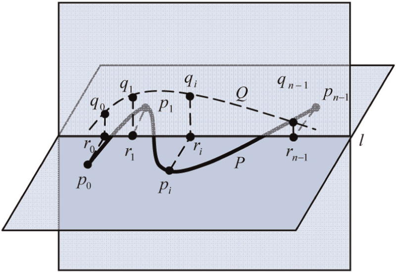
Calculation of interpolated point.
Offset and offset point
Assume that the original stroke is located in the xz plane, for example, and the normal of plane is along the y-axis. The coordinate of
The coordinate of offset point

Offset point.
Creation of spatial stroke
The spatial stroke can be created using the data in the array
First, two strokes are selected from the stack of stroke set, which are marked as highlight for 3D stroke fitting;
Second, the location relationship of two strokes is judged to determine whether the two planes are orthogonal ones or not. If so, 3D stroke fitting is processed. Otherwise, the algorithm is stopped;
Third, the lengths of two strokes are calculated, and the interval is determined and then the interpolating points and offset points are calculated;
Finally, if 3D fitting is successful, all of the offset points are used to draw a B-spline stroke (as shown in Figure 7).

3D stroke after fitting.
Test of the fitting algorithm
Here gives an example to demonstrate the 3D stroke fitting in two orthogonal planes (as shown in Figure 8). Some strokes are sketched at first on the screen plane N and then they are combined together as the original stroke (as shown in Figure 8(a) and (b)). The screen plane N is rotated and overlapped with the plane M, so that the original stroke is located in the plane M. Some new strokes are sketched again in the screen plane N (as shown in Figure 8(c)) and then they will be joined together as the modifying stroke. The modifying stroke in the plane N and the original stroke in the plane M are used to create a 3D stroke (as shown in Figure 8(d)). If changing the modifying stroke further by drawing some new strokes in the plane N (as shown in Figure 8(e)), the final 3D stroke will be improved at the same time (as shown in Figure 8(a) and (f)). The algorithm works well when strokes are simple and not closed. But the ambiguous results will occur sometimes for the closed strokes. Therefore, the projective algorithm has been applied to deal with the case. Only the parallel projection is taken into account in the stroke fitting.

Offset point: (a) sketching strokes, (b) stroke after combination, (c) switch the working plane, (d) 3D stroke fitting, (e) modify further, and (f) new 3D stroke.
Stroke fitting based on projection
Stroke based on orthographic projection
The relationship of the stroke and the projective plane is orthogonal (as shown in Figure 9(a)). Assume that the stroke P is a set of points


Stroke fitting based on the projection: (a) orthographic projection and (b) oblique projection.
According to the relationship of orthogonal projection, there are

For a given equation
Therefore, the coefficients are

The point
where

Stroke based on oblique projection
It is a kind of parallel projection, but the projection plane is not perpendicular to the projective ray. Orthographic projection can be interpreted as a kind of oblique projection along the normal. Similarly, its projection plane M is defined by Q and

The projective stroke S in parametric pattern is
The relationship between the freehand sketching plane and the projective stroke plane is restricted by orthographic projection. If sketching in one plane in the world coordinate system, the projection of the stroke is done only along its normal direction. However, oblique projection is relatively flexible and the stroke projection can be done by the vector transformation on any projection plane.
Lofting
It is a kind of method of surface construction based on the projection, in which the surface is modified by a spline. 17 The stroke is drawn in a plane and then modified by a spline to form a spatial stroke. Here, the screen plane is considered as the projective plane M, and the projective stroke as a spline for lofting to create surfaces (yellow ones as shown in Figure 9(a) and (b)). The procedure of surface construction is as follows:
First, it needs to find out a sectional stroke, which is a planar and defined under the screen coordinate system. The values of vertices can be calculated through a set of points obtained by the Newton method in the orthographic or oblique projective stroke and then the control vertices will be calculated by the reverse mapping;
Second, it is to find out a spline, which is planar or spatial. Here, the projective direction should be determined, and the end vertex is considered as the point, the target point, transformed from the screen plane to space. Obviously, the target point is located within the projection plane but not necessarily on the sectional stroke. The spline reflects the shape of the vertical distribution of the loft surface, so that the node vector of the spline coincides with the one on the surface, in the longitudinal direction;
Third, the sectional stroke is translated to space until the origin and the target points are overlapped. In orthographic projection, the sectional stroke has been located within the normal plane because the spline is the normal vector of the projective plane, that is, the screen plane. For oblique projection, the sectional stroke should be rotated to the normal plane at the target point of the spline. According to the geometrical invariability, the transformation is conducted only for the B-spline control points of sectional stroke;
Finally, the lofting surface is created according to those B-spline control points after the reverse mapping.
Create 3D stroke
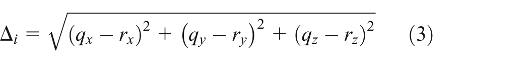
A 3D stroke will be created to realize the fitting of 3D stroke through the projection of an original stroke on the lofting surface, which is lofted by a sectional stroke along a spline. The fitting process is understood to find the interpolation points
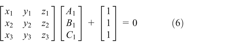
A surface

and it meets the condition: the straight line

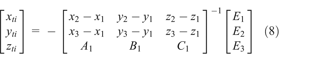
The closest points are available by solving the equations. Similar to the issue encountered with the orthographic projection, the Newton iterative method is applied. Through the evaluation of distributed point on the surface, the parameter


where


In the ith step of Newton iteration, the matrix equation of

Similar to the discussion in section “Stroke based on orthographic projection,” the checking conditions are stated as follows:
The overlapped point is checked according to
The zero cosine is checked to make it perpendicular between

If either of these two conditions is not met, then the iteration is continued, and two additional conditions are checked as follows: whether the parameters are located between the domains

If this condition is met, then the iteration is over. The current parameter
Examples of projective fitting
Here are some examples of 3D stroke fitting based on the projection realized in AutoSketch. The first example is to sketch a line (after the stroke standardization of stroke) on the screen plane N (as shown in Figure 10(a)) and switch it into the plane M, which is perpendicular to the screen plane N. The projection of the line on the screen plane N is still a straight line (as shown in Figure 10(b)). It will be modified by sketching some strokes to form a new modifying stroke, which is to change reversely the shape of the line. Therefore, the line becomes a stroke, which is still a planar one and is located in the plane P (as shown in Figure 10(c)).

Projective fitting of a line: (a) original stroke, (b) projection of line, and (c) 3D stroke created.
The next two examples show that the closed stroke fitting in 3D. A closed triangle is drawn by sketching three strokes (after the geometric standardization of stroke) on the screen plane N (as shown in Figure 11(a)). It is switched into the plane M, and its projective line on the screen plane N is still a straight line (as shown in Figure 11(b)). Modifying the projective line by sketching some new strokes can form a new modifying stroke (as shown in Figure 11(c)) and then the planar triangle is bent into the spatial triangle. Similarly, a closed circle can be obtained by sketching one or some strokes on the screen plane N (as shown in Figure 12(a)). The screen plane N is then flipped into the plane M in a different way (as shown in Figure 12(b)). The projection of the circle on the screen plane is also a straight line. It can be modified and then to modify the circle actually to make it become a spatial stroke (as shown in Figure 12(c)).

Projective fitting of a closed triangle: (a) a closed triangle, (b) projection of triangle, and (c) 3D triangle created.

Projective fitting of a closed circle: (a) original stroke, (b) projective stroke, and (c) 3D stroke created.
The last example demonstrates how to sketch a lamp frame or outlines of vehicle. At first, a working plane is defined, which may be the screen plane N or a plane W (as shown in Figure 13(a)) in the front 3/4 view, for instance, so that the strokes drawn on the screen N are actually drawn on the working plane W. The strokes was smoothed and processed to form a closed planar outline of lamp (as shown in Figure 13(b) and (c)). The working plane is turned into another view (as shown in Figure 13(d)), and a modifying stroke is sketched to bend the frame of lamp (as shown in Figure 13(e)). Now the frame of lamp is a spatial one to meet the actual requirement of automotive styling (as shown in Figure 13(f)), and then the surface of lamp is created according to the frame. Some details are added to complete the design of lamp (as shown in Figure 13(g)–(i)).
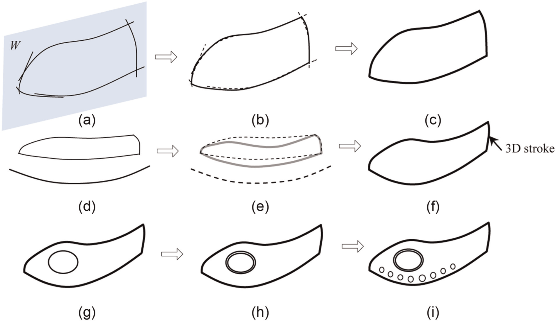
Sketching a lamp frame: (a) strokes on the plane W, (b) stroke processing, (c) closed frame of lamp in 2D, (d) sketch a modifying stroke, (e) curved frame of lamp, (f) 3D frame of lamp, (g) sketch on the surface of lamp, (h) add the details, and (i) add some ornaments.
Orthographic resultant method
Algorithm
In the freehand sketching, the drawing deviation is unavoidable. A mathematical model of surface intersection is built at first in order to make an accurate expression of the position of the intersection stroke. The calculation process of 3D reconstruction is degraded; the spatial stroke is projected onto the screen plane and then is fitted in real time to realize the fitting of its original spatial stroke.
The convex hull construction of spatial stroke is the basis for calculating interpolation of the spatial intersection stroke. The idea of incremental algorithm of calculating the convex hull in 2D space is extended to 3D one. Unlike in 2D space, the data structure of convex hull in 3D space is composed of vertices, edges, and surface, which also allows adding or deleting each element.
The incremental algorithm of convex hull in 3D is similar to it in 2D. Each scattered spatial data point will be processed and combined with the previous point within the convex hull. All the coplanar points can produce a planar convex polygon in 2D, and the convex hull in 3D is considered as a cone (as shown in Figure 14). The visible surface must be removed from the current convex hull and the surface of cone must be added.
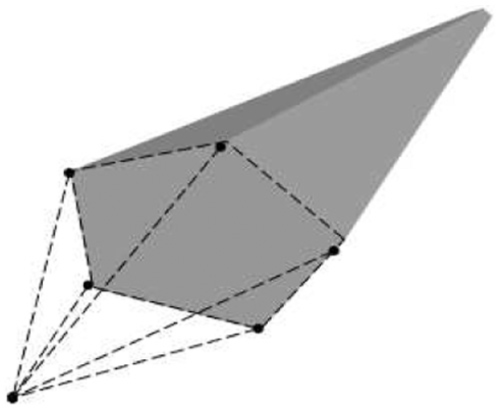
Current convex hull of spatial points.
A spatial surface is composed of convex hull data points, which is presented by the strokes corresponding to nodes with the same parameters in the u and v directions (as shown in Figure 15). A local change of a surface patch will occur when the stroke is changed in the u or v parametric direction. It shows that the purpose of changing the surface shape can be achieved by changing the shape of the parametric strokes.

Local changes of a surface patch.
The projective stroke in the xy, yz, or xz plane can be obtained, respectively, through the projection of a spatial stroke along the axial direction. The shapes of projective strokes are different. The extended surface can be obtained easily by expanding the projective stroke along the normal of the projective plane (as shown in Figure 16(a) and (b), where S is the spatial stroke and
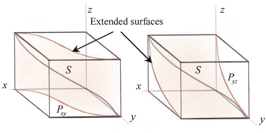
Extended surfaces.
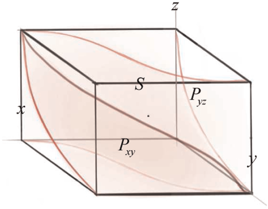
Intersection of extended surfaces.
From a mathematical point of view to solve the problem of computer graphics, solving the intersecting curve of two surfaces can be understood as follows: the ternary simultaneous equations with the higher order of the two surfaces are built at first, and the equations are eliminated. The two coordinate parameters left represent the orthographic projection of surface on the projective plane.
The concept of resultant is introduced here to solve the problem above. The definition of resultant is as follows: for two polynomials

the determinant of coefficient is

which is called the resultant of polynomials
Resultant theorem
Assume that there is one indeterminate in the polynomials in equation (18) and
The theorem is very important to deal with the problem discussed above. Assume that
with all solutions in the domain of real numbers so that

where

Solving shows that if
From the point of view of geometric mathematics,

where

Similarly, if the root
The geometric meaning of the mathematical model is:
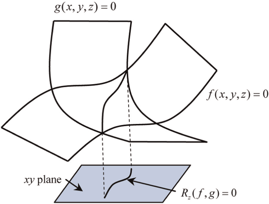
Geometric meaning of resultant method.
Examples
The algorithm above was applied in AutoSketch system and tested. Here gives an example of 3D stroke creation.
Some strokes (the dotted ones as shown in Figure 17(a)) are sketched on the screen plane N, which is the working plane currently. They are joined together through the combination algorithm 11 into a smooth stroke (the orange stroke as shown in Figure 19(a)). This is the first stroke for 3D stroke creation, which is located in the xy plane and will not be changed later on after switching the working plane on the floor (as shown in Figure 19(b)). Now the working plane and the screen plane N are perpendicular to each other. An extended virtual surface is created by giving an extending vector (the positive z-axis is used here as show in Figure 19(c)) and then is pointed as the new working plane (a surface). Now some new strokes (dotted ones as shown in Figure 19(d)) are sketched on the screen plane N and combined as the second stroke (yellow one as shown in Figure 19(e)) for 3D stroke creation, which is located in the xz plane. The projective stroke of the second stroke is on the working plane, which is fitted by the first and the second strokes (green one as shown in Figure 19(f)). It looks like sketching directly on the working surface while sketching the second stroke, because they are overlapped while looking the screen. The projective stroke is an actual required 3D stroke. If modifying the second stroke further, new modifying stroke(s) can be drawn on the screen plane N (dotted ones as shown in Figure 19(g)) and then the second stroke is changed in shape (brown one as shown in Figure 19(h)). The 3D stroke is also changed at the same time (pink one as shown in Figure 19(i)). This example shows a typical case. In general, the extending vector can be in any direction. Therefore, the extending surface may be changed.

First stroke created in AutoSketch: (a) multi-strokes and their combination, (b) change the working plane, (c) an extended surface created, (d) new multi-strokes sketched on the screen, (e) combined to a new stroke, (f) its projective stroke on the working plane, (g) new stroke for modification, (h) the new stroke changed, and (i) projective stroke changed then.
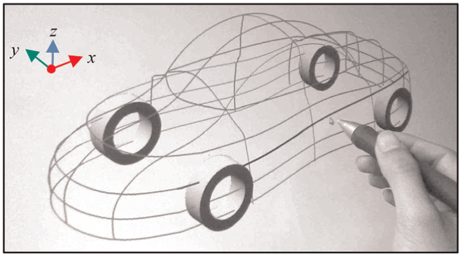
Another example shows how to draw a side waist outline of vehicle. A stroke is sketched first in the xy plane in the current working coordinate system and selected with highlight in red (as shown in Figure 20). If it needs to be modified in the z direction, the current working plane is set to be parallel to the plane xz, and a modifying stroke is sketch on it (green one as shown in Figure 21). Therefore, the new 3D stroke is created (as shown in Figure 22). This is a spatial waist outline that meets the curve features of automotive styling.
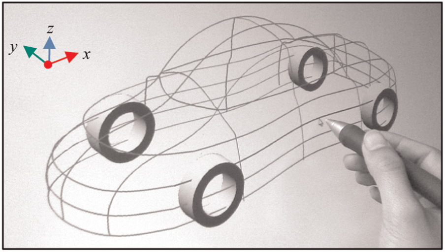
Choose a smooth stroke on the plane xy.

Draw the modifying stroke.
New 3D stroke after fitting.
Conclusion
The research has discussed three issues to create 3D stroke based on the previous studies in the planar stroke combination algorithms developed. The first algorithm of 3D stroke fitting is realized by calculating simply the interpolation points of two strokes, which are located in two orthogonal planes. This algorithm is suitable for the simple strokes. It does not work well for the closed strokes. Therefore, the second one has been developed to work well with the case. It creates 3D stroke by the projection of two strokes in two orthogonal planes and the lofting. The third one has investigated the 3D stroke obtained from the intersecting stroke or curve of two surfaces. It projects a spatial stroke onto the screen plane to get a projective stroke, which is modified on the screen, and then the original spatial stroke is changed reversely by intersection. Three methods have been prototyped in AutoSketch system. Comparing three algorithms, the first one is simple and easy to calculate, the second one is suitable for more cases, and the third one gives a more general solution. However, the reliability and availability of algorithms need to be improved further.
Footnotes
Academic Editor: Michal Kuciej
Declaration of conflicting interests
The authors declare no conflict of interests.
Funding
This work was supported by the Science and Technology Plan Projects of Zhejiang Province under grant no. 2013C31085 for project “3D-sketching automotive styling system based on pressure-sensitive and pen strokes convergence technology”, and the Science and Technology Plan Projects of Jinhua City under the grant no. 2011-1-045 for project “research on way of automotive styling input 3D-sketching”.