Monitoring vertical wheel–rail contact forces based on freight wagon inverse modelling

Abstract

The safety and stability of freight train operations are closely related to the wheel–rail contact dynamic forces. To evaluate and monitor the wheel–rail dynamic forces based on the accelerations on the wagon components, a two-dimensional inverse wagon model has been developed. To verify the inverse modelling, a detailed VAMPIRE wagon model has been used for the simulations on two cases of track rail top surface and cross-level irregularities. The simulated accelerations on wagon components are then the inputs into the inverse wagon model. Reasonable agreement has been achieved in the comparison between the predicted and simulated primary and secondary suspension forces and wheel–rail contact forces. The inverse wagon model is finally simplified into a one-dimensional vertical model for potential online applications. The predicted and simulated wheel–rail contact dynamic forces are also compared due to the random track geometry irregularities.

Introduction

The railway vehicles generate and are subjected to dynamic forces when they run on tangential or curved tracks with geometry irregularities. The excessive dynamics of the vehicle–track system leads to severe impact of wheel on the railhead and wheel unloading (WU) with derailment potential. Depending on the track geometry irregularities, significant dynamic forces occur in the vertical directions. Simultaneous occurrence of the vertical dynamic loading has the potential to severely damage the rails and the wheels, or the potential to cause the derailments.

Understanding the freight wagon dynamic behaviour, for example, wheel–rail (WR) dynamic forces, is very important for the freight train operations. Currently, the accelerations on wagon components can be easily obtained due to the excellent range of transducers available. The problem is how to predict WR dynamic forces based on the wagon responses. In fact, such a problem belongs to one of the inverse dynamics identification problems. The inverse identification problem can be defined as finding system inputs based on given responses, boundary conditions and system modelling. Inverse identification problems are of paramount importance for monitoring and quality control purposes arising in critical applications in engineering.^1–5 Mathematical modelling and the numerical study of these problems require high competence in computational mechanics and applied optimisation. To solve the inverse identification problem, an inverse model of the system has to be known.

The limited applications of inverse identification problems in vehicle–track systems are reviewed as follows. The method based on Tikhonov’s regularisation ⁶ was applied to the identification of WR contact forces based on the axle box accelerations. Meanwhile, the theoretical background and main limits to the application of inverse identification methods were discussed. Numerical and experimental tests on a laboratory rig were made to verify the formulated procedures. An inverse wagon model^7–9 was developed to estimate WR contact forces using only measurements of wagon body responses as inputs. The model combines integration and partial modal matrix techniques. Besides WR contact forces, some motion quantities such as the lateral and yaw displacements of wheelset are also predicted. In order to estimate the high-frequency components of the forces at the WR interface due to suspension, a grey box-based inverse wagon model ¹⁰ was developed. The high-frequency forces may be considered as the responses to random track irregularities with high frequency and appear as a random feature. A recurrent neural network (RNN) architecture ¹¹ has been proposed to predict the WR interface dynamics due to short wavelength defects. The architecture proposed was found to converge quickly during the training process and predict the output in the form of a vertical force factor quite well in comparison to the simulated results.

A method based on an Auto-Regression model with eXtra inputs (ARX) ¹² was used to estimate track geometry irregularities by measuring accelerations of a passenger car instead of direct measurement by using a conventional track inspection car. The quality of the estimation is evaluated quantitatively by using the mean square error. The effects due to two major uncertainties, mass variations and speed variations, are evaluated by using the singular value decomposition in order to present the limitations of the estimation using a nominal model. A method for track geometry assessment considered the vehicle–track interaction. ‘Representative’ transfer functions are used for the prediction of the vehicle reaction. Therefore, the results showed a significant enhancement of the correlation between the track assessment quantities and the vehicle response forces. ¹³ A structural health monitoring system was developed based on vibration measurements during the rail vehicle operation simultaneously with global positioning system (GPS) position and velocity estimation. An algorithm for rail track health assessment is formulated as an inverse identification problem of dynamic parameters of the rail vehicle system. Track irregularities are identified using this procedure. ¹⁴

Monitoring the WR dynamic forces is very important for railway operations. Currently, the acceleration transducers on rail vehicle components are easily installed and maintained for the railway industry. The possibility of establishing a relationship between the WR dynamic forces and the accelerations on wagon components has been theoretically worked out in this article. The research has been, at first, carried out on case studies due to a rail top surface and a cross-level irregularity using a very detailed wagon model generated using VAMPIRE package. Then, an inverse wagon model has been developed to predict the dynamic forces between the wagon component connections, the wheel and rail contact forces based on the accelerations from the VAMPIRE wagon model. The prediction calculations were carried out by using a numerical integration modified Newmark-β method. ¹⁵ The predicted outputs – dynamic forces – have been compared with those directly available from the detailed VAMPIRE model. In the article, the inverse wagon model will be described in detail. The comparison between the simulations and the predictions will be illustrated and discussed.

Wagon dynamics inverse modelling

The two-dimensional (lateral and vertical) wagon dynamic inverse modelling is shown in Figure 1(a) and (b).

Figure 1.

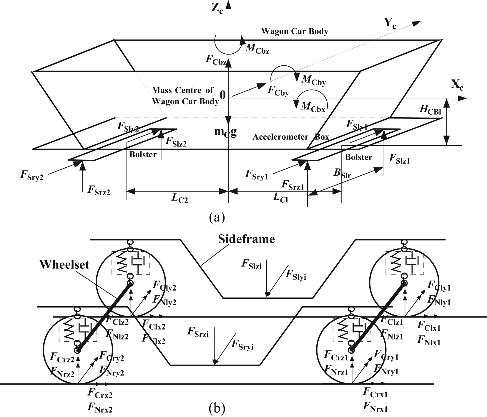
Inverse wagon modelling: (a) wagon car body and (b) bogie.

The inverse modelling can be described as following steps:

• The determination of secondary suspension (SS) forces. In this article, for the accelerations of the wagon car body and two bogie sideframes (SFs) at the SS positions, respectively, the double integrations are carried out to obtain the velocities and displacements. Therefore, the SS forces can be determined by multiplying the damping and stiffness coefficients of the suspension springs and dampers by the relative velocity and displacement.

• The dynamic equilibrium equations are established for the bogie SFs and wheelsets. Such a dynamic system is subjected to the so-called external forces – the SS forces.

• A numerical method is applied to solve the system equations. Finally, the primary suspension (PS) and WR contact forces can be determined.

The determination of PS and SS forces is based on the explicit Kelvin–Voigt model in which a viscous damper and an elastic spring are connected in parallel, instead of the Maxwell model where two elements are connected in series, or other generalised models. This is because the PS and SS in rail vehicles are generally made of flexi coil springs and as such will have coupled lateral and vertical behaviours; also, there is the internal damping of a coil spring, which exists to some extent in the materials experiencing deflection, and the damping force is dependent only upon the relative velocity experienced by both ends of the spring. Therefore, a viscous damper and an elastic spring are connected in parallel.

The flowchart for the above inverse modelling can be shown in Figure 2:

Figure 2.

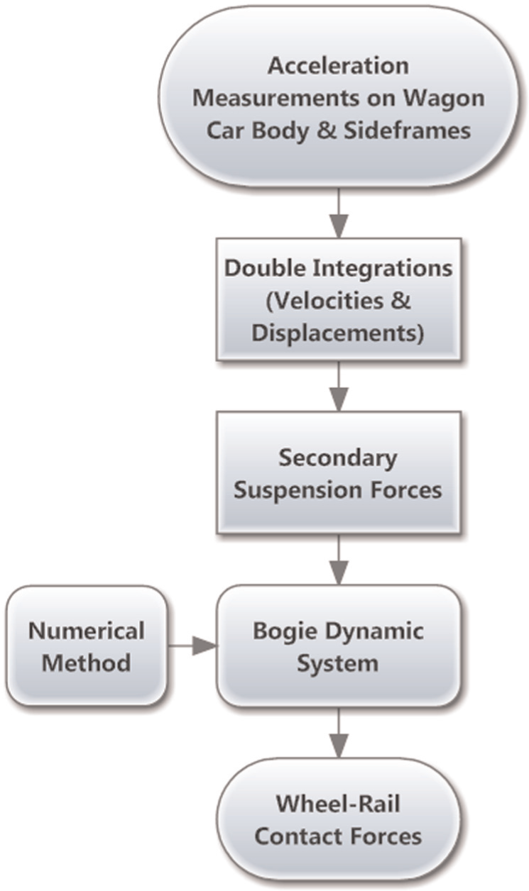
Flowchart.

Bogie SF

Three degrees of freedom (DoFs) describing the motions of the bogie SF, namely, the lateral and vertical displacements ( $v_{\mathrm{sf}}$ and $w_{\mathrm{sf}}$ ) and the pitch rotations ( ${\varnothing }_{\mathrm{By}}$ ) about the $X_B$ , $Y_B$ and $Z_B$ axes are used. In Figure 1(b), the dynamic equivalent equations of SFs on each bogie (i = 1, 2) can be written as

$$\begin{array}{cc}\multicolumn{1}{c}{}& \mathrm{The}\mathrm{left}\mathrm{sideframe}:\hfill \\ \multicolumn{1}{c}{}& \{\begin{array}{c}\hfill m_{\mathrm{Sf}}\underset{\mathrm{Sfli}}{\stackrel{··}{v}}=F_{\mathrm{Plyi}1}+F_{\mathrm{Plyi}2}-F_{\mathrm{Slyi}}\hfill \\ \multicolumn{1}{c}{m_{\mathrm{Sf}}\underset{\mathrm{Sfli}}{\stackrel{··}{w}}=F_{\mathrm{Plzi}1}+F_{\mathrm{Plzi}2}-F_{\mathrm{Slzi}}}\\ \multicolumn{1}{c}{J_{\mathrm{Sfy}}\underset{\mathrm{Sflyi}}{\stackrel{··}{\varnothing }}=H_{\mathrm{wSf}}(F_{\mathrm{Plxi}1}+F_{\mathrm{Plxi}2})+L_w(F_{\mathrm{Plzi}2}-F_{\mathrm{Plzi}1})}\end{array}\hfill \end{array}$$

(1)

$$\begin{array}{cc}\multicolumn{1}{c}{}& \mathrm{The}\mathrm{right}\mathrm{sideframe}:\hfill \\ \multicolumn{1}{c}{}& \{\begin{array}{c}\hfill m_{\mathrm{Sf}}\underset{\mathrm{Sfri}}{\stackrel{··}{v}}=F_{\mathrm{Pryi}1}+F_{\mathrm{Pryi}2}-F_{\mathrm{Sryi}}\hfill \\ \multicolumn{1}{c}{m_{\mathrm{Sf}}\underset{\mathrm{Sfri}}{\stackrel{··}{w}}=F_{\mathrm{Przi}1}+F_{\mathrm{Przi}2}-F_{\mathrm{Srzi}}}\\ \multicolumn{1}{c}{J_{\mathrm{Sfy}}{\stackrel{··}{\varnothing }}_{\mathrm{Sfryi}}=H_{\mathrm{wSf}}(F_{\mathrm{Prxi}1}+F_{\mathrm{Prxi}2})+L_w(F_{\mathrm{Przi}2}-F_{\mathrm{Przi}1})}\end{array}\hfill \end{array}$$

(2)

in which $m_{\mathrm{Sf}}$ and $J_{\mathrm{Sfy}}$ are the SF mass and mass inertia moment about $Y_B$ axis, $F_S$ and $F_P$ represent the SS and PS forces, $H_{\mathrm{wSf}}$ is the height between wheelset axle box and the mass centre of SF and $L_w$ is the longitudinal distance between two wheelsets in a bogie.

Wheelset

Four DoFs describing the motions of a wheelset, namely, the lateral and vertical displacements ( $v_W$ and $w_W$ ) and the roll and the yaw rotations ( ${\varnothing }_{\mathrm{Bx}}$ and ${\varnothing }_{\mathrm{Bz}}$ ) about the $X_W$ and $Z_W$ axes. In Figure 1(b), the dynamic equivalent equations of each wheelset (i = 1 and 2; j = 1 and 2) can be written as

$$\left[\begin{array}{cccc}\hfill m_W\hfill & \hfill 0\hfill & \hfill 0\hfill & \hfill 0\hfill \\ \multicolumn{1}{c}{0}& \hfill m_W\hfill & \hfill 0\hfill & \hfill 0\hfill \\ \multicolumn{1}{c}{0}& \hfill 0\hfill & \hfill J_{\mathrm{Wx}}\hfill & \hfill 0\hfill \\ \multicolumn{1}{c}{0}& \hfill 0\hfill & \hfill 0\hfill & \hfill J_{\mathrm{Wz}}\hfill \end{array}\right]\left\{\begin{array}{c}\hfill \begin{array}{c}\hfill \underset{\mathrm{Wij}}{\stackrel{··}{v}}\hfill \\ \multicolumn{1}{c}{\underset{\mathrm{Wij}}{\stackrel{··}{w}}}\end{array}\hfill \\ \multicolumn{1}{c}{\begin{array}{c}\hfill \underset{\mathrm{Wxij}}{\stackrel{··}{\varnothing }}\hfill \\ \multicolumn{1}{c}{\underset{\mathrm{Wzij}}{\stackrel{··}{\varnothing }}}\end{array}}\end{array}\right\}=\left\{\begin{array}{c}\hfill \begin{array}{c}\hfill F_{\mathrm{PWyij}}\hfill \\ \multicolumn{1}{c}{F_{\mathrm{PWzij}}}\end{array}\hfill \\ \multicolumn{1}{c}{\begin{array}{c}\hfill M_{\mathrm{PWxij}}\hfill \\ \multicolumn{1}{c}{M_{\mathrm{PWzij}}}\end{array}}\end{array}\right\}$$

(3)

$$\begin{array}{cc}\multicolumn{1}{c}{}& \left[M_W\right]\left\{{\stackrel{··}{q}}_{\mathrm{Wij}}\right\}=\left\{F_{\mathrm{PWij}}\right\}(i=1,2\mathrm{and}j=1,2)\hfill \\ \multicolumn{1}{c}{}& \left\{\begin{array}{c}\hfill \begin{array}{c}\hfill F_{\mathrm{PWyij}}\hfill \\ \multicolumn{1}{c}{F_{\mathrm{PWzij}}}\end{array}\hfill \\ \multicolumn{1}{c}{\begin{array}{c}\hfill M_{\mathrm{PWxij}}\hfill \\ \multicolumn{1}{c}{M_{\mathrm{PWzij}}}\end{array}}\end{array}\right\}=\left\{\begin{array}{c}\hfill \begin{array}{c}\hfill -F_{\mathrm{Plyij}}-F_{\mathrm{Pryij}}+F_{\mathrm{Clyij}}+F_{\mathrm{Cryij}}\hfill \\ \multicolumn{1}{c}{-F_{\mathrm{Plzij}}-F_{\mathrm{Przij}}+F_{\mathrm{Nlzij}}+F_{\mathrm{Nrzij}}}\end{array}\hfill \\ \multicolumn{1}{c}{J_{\mathrm{Wy}}\frac{V}{r_0}{\stackrel{·}{\varnothing }}_{\mathrm{Wzij}}-r_0(F_{\mathrm{Clyij}}+F_{\mathrm{Cryij}})+B_{\mathrm{Wlr}}(F_{\mathrm{Nrzij}}-F_{\mathrm{Nlzij}})+B_{\mathrm{Plr}}(F_{\mathrm{Plzij}}-F_{\mathrm{Przij}})}\\ \multicolumn{1}{c}{-J_{\mathrm{Wy}}\frac{V}{r_0}{\stackrel{·}{\varnothing }}_{\mathrm{Wxij}}+B_{\mathrm{Wlr}}(F_{\mathrm{Clxij}}-F_{\mathrm{Crxij}})+B_{\mathrm{Wlr}}{\varnothing }_{\mathrm{Wzij}}(F_{\mathrm{Clyij}}-F_{\mathrm{Cryij}})}\end{array}\right\}\hfill \end{array}$$

(4)

In equations (3) and (4), $m_W$ , $J_{\mathrm{Wx}}$ and $J_{\mathrm{Wz}}$ are the wheelset mass and mass inertia moment about $X_W$ and $Z_W$ axes, $F_N$ and $F_C$ represent the WR contact normal forces and creep forces, $V$ is the wagon speed, $r_0$ is the wheel radius and $B_{\mathrm{Wlr}}$ is the lateral distance between the WR contact point and the track centreline.

WR contact forces

The WR normal forces ( $F_N$ ) can be determined by the following equation

$$\{\begin{array}{c}\hfill F_{\mathrm{Nlzij}}=C_H{[(w_{\mathrm{Wij}}-B_{\mathrm{Wlr}}{\varnothing }_{\mathrm{Wxij}})-{\mu }_l\left(x\right)]}^{3/2},\mathrm{if}[(w_{\mathrm{Wij}}-B_{\mathrm{Wlr}}{\varnothing }_{\mathrm{Wxij}})-{\mu }_l\left(x\right)]\le 0,F_{\mathrm{Nlzij}}=0\hfill \\ \multicolumn{1}{c}{F_{\mathrm{Nrzij}}=C_H{[(w_{\mathrm{Wij}}+B_{\mathrm{Wlr}}{\varnothing }_{\mathrm{Wxij}})-{\mu }_r\left(x\right)]}^{3/2},\mathrm{if}[(w_{\mathrm{Wij}}+B_{\mathrm{Wlr}}{\varnothing }_{\mathrm{Wxij}})-{\mu }_r\left(x\right)]\le 0,F_{\mathrm{Nrzij}}=0}\end{array}$$

(5)

in which $C_H$ is Hertz contact coefficient and $\mu (x)$ are the track irregularities.

For the longitudinal and lateral tangent creep forces, the Kalker’s linear theory is applied. ¹⁶ Due to the elasticity of wheel and rail, some areas on the contact surface may slip while others may stick when a wheel is rolling on a rail because the difference between the tangential strains of two bodies in the adhesion area leads to small apparent slip (creepage). Creepages generate tangential creep forces and spin moment on the WR contact surface since the motion of the wheel relative to the rail is a combination of rolling and sliding. In 1968, Kalker introduced the theory which defined the relationship between the creepages and the creep forces. They are simply expressed as (ignorance of spin creep)

$$\begin{array}{cc}\multicolumn{1}{c}{}& \{\begin{array}{c}\hfill f_{\mathrm{Clxj}}=-f_{33}{\epsilon }_{\mathrm{lxj}}=-f_{33}(B_{\mathrm{Wlr}}\frac{{\stackrel{·}{\varnothing }}_{\mathrm{Wzij}}}{V}+\frac{\lambda y}{r_0})\hfill \\ \multicolumn{1}{c}{f_{\mathrm{Crxj}}=-f_{33}{\epsilon }_{\mathrm{rxj}}=-f_{33}(-B_{\mathrm{Wlr}}\frac{{\stackrel{·}{\varnothing }}_{\mathrm{Wzij}}}{V}-\frac{\lambda y}{r_0})}\end{array},\hfill \\ \multicolumn{1}{c}{}& \{\begin{array}{c}\hfill f_{\mathrm{Clyj}}=-f_{11}{\epsilon }_{\mathrm{lyj}}=-f_{11}(\frac{{\stackrel{·}{v}}_{\mathrm{Wij}}}{V}-{\varnothing }_{\mathrm{Wzij}})\hfill \\ \multicolumn{1}{c}{f_{\mathrm{Cryj}}=-f_{11}{\epsilon }_{\mathrm{ryj}}=-f_{11}(\frac{{\stackrel{·}{v}}_{\mathrm{Wij}}}{V}-{\varnothing }_{\mathrm{Wzij}})}\end{array},\hfill \end{array}$$

(6)

in which $f_{11}$ and $f_{33}$ are the creep coefficients, $\epsilon$ and $f_C$ represent the creepage and creep force.

Kalker’s linear theory is limited to the case of small creepages. For the determination of creep forces, they are first computed by using Kalker’s linear theory, and the nonlinear effect of adhesion limit is included by computing a resultant force $f_{\mathrm{re}}$ as follows

$$f_{\mathrm{rej}}=\sqrt{f_{\mathrm{Cxj}}^2+f_{\mathrm{Cyj}}^2}$$

(7)

According to Coulomb friction law, the magnitude of the resultant creep force cannot exceed the pure slip value ${\mu }_k{F}_{\mathrm{Nj}}$ . Using Johnson and Vermeulen’s theory ¹⁶ for creep without spin, the resultant force $f_{\mathrm{rej}}$ is limited by the nonlinear value $\overline{f_{\mathrm{rej}}}$ as follows

$$\begin{array}{cc}\multicolumn{1}{c}{}& \overline{f_{\mathrm{rej}}}=\hfill \\ \multicolumn{1}{c}{}& \{\begin{array}{cc}\hfill {\mu }_k{F}_{\mathrm{Nj}}[\frac{f_{\mathrm{rej}}}{{\mu }_k{F}_{\mathrm{Nj}}}-\frac{1}{3}{\left(\frac{f_{\mathrm{rej}}}{{\mu }_k{F}_{\mathrm{Nj}}}\right)}^2+\frac{1}{27}{\left(\frac{f_{\mathrm{rej}}}{{\mu }_k{F}_{\mathrm{Nj}}}\right)}^3]\hfill & \hfill \mathrm{for}{f}_{\mathrm{rej}}\le 3{\mu }_k{F}_{\mathrm{Nj}}\hfill \\ \multicolumn{1}{c}{{\mu }_k{F}_{\mathrm{Nj}}}& \hfill \mathrm{for}{f}_{\mathrm{rej}}>3{\mu }_k{F}_{\mathrm{Nj}}\hfill \end{array}\hfill \end{array}$$

(8)

in which ${\mu }_k$ is the coefficient of friction at the WR contact and $F_{\mathrm{Nj}}$ is the normal force at the WR contact.

For small creepages, when $f_{\mathrm{rej}}\le 3{\mu }_k{F}_{\mathrm{Nj}}$ , the creep forces are determined by

$$F_{\mathrm{Cxj}}=\frac{f_{\mathrm{Cxj}}}{f_{\mathrm{rej}}}\overline{f_{\mathrm{rej}}},F_{\mathrm{Cyj}}=\frac{f_{\mathrm{Cyj}}}{f_{\mathrm{rej}}}\overline{f_{\mathrm{rej}}}$$

(9)

For complete slip, when $f_{\mathrm{rej}}>3{\mu }_k{F}_{\mathrm{Nj}}$ , the creep forces are as below

$$F_{\mathrm{Cxj}}=\frac{{\epsilon }_{\mathrm{xj}}}{\sqrt{{\epsilon }_{\mathrm{xj}}^2+{\epsilon }_{\mathrm{yj}}^2}}{\mu }_k{F}_{\mathrm{Nj}},F_{\mathrm{Cyj}}=\frac{{\epsilon }_{\mathrm{yj}}}{\sqrt{{\epsilon }_{\mathrm{xj}}^2+{\epsilon }_{\mathrm{yj}}^2}}{\mu }_k{F}_{\mathrm{Nj}}$$

(10)

Based on equations (1)–(10), the dynamic equivalent equations of an inverse wagon model can be written in the matrix form as

$$\left[M_w\right]\left\{{\stackrel{··}{q}}_w\right\}+\left[C_w\right]\left\{{\stackrel{·}{q}}_w\right\}+\left[K_w\right]\left\{q_w\right\}=\left\{F_w\right\}$$

(11)

in which $[M_w]$ , $[C_w]$ and $[K_w]$ are the mass, damping and stiffness matrixes of inverse wagon modelling. $\{q_w\}$ and $\{F_w\}$ are the displacement vector and the force vector. The total of DoFs is 28. In equation (11), the SS forces are known. Therefore, through equation (11), the WR contact forces can be predicted through calculations using a modified numerical integration Newmark-β method. ¹⁵

Wagon dynamics modelling using VAMPIRE

Rail vehicle dynamics have been widely investigated using the VAMPIRE software. ¹⁷ In this section, a wagon model is generated using VAMPIRE, and two track geometry irregularities – top surface and cross level – are selected for the simulations.

VAMPIRE wagon modelling

A wagon model generated using VAMPIRE package is shown in Figure 3.^18,19 The wagon model in Figure 3 contains 11 masses (1 wagon car body, 2 bolsters, 4 SFs and 4 wheelsets). The connections among these 11 masses have been modelled using 17 stiffness elements, 74 bumpstop elements, 13 viscous damper elements, 116 friction elements and 4 shear spring elements, which fully consider the nonlinear characteristics of the connections. The wagon data for the VAMPIRE simulations and the inverse modelling predictions are given in Appendix 1.

Figure 3.

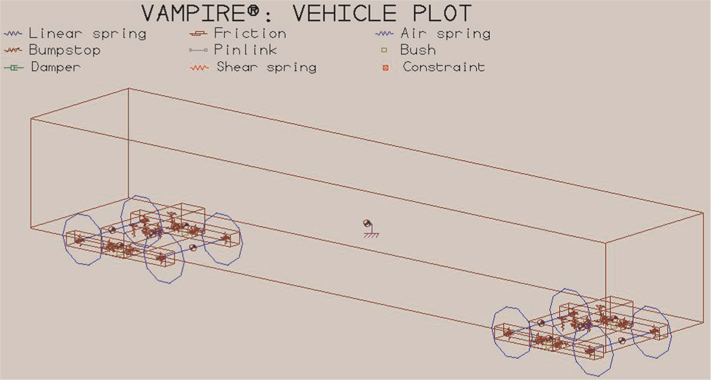
VAMPIRE wagon model.

It will be noticed that the validation of inverse dynamic wagon model is highly dependent upon the direct dynamic wagon model that has been generated using VAMPIRE software, as shown in Figure 3. The various analysis techniques used in VAMPIRE for vehicle dynamic predictions were each validated in a series of track tests in the late 1970s and early 1980s. Also, a number of benchmark exercises like Manchester Benchmark have been undertaken for the various validations. In general, excellent agreement has been shown between the various comparisons, with the differences being attributable to variations between the parameters used. The wagon model therefore can be considered sufficiently validated for the purpose of this article.

Track geometry irregularities

The track geometry irregularities in the case studies are shown in Figure 4(a) and (b). Case 1 is a top surface with a length of 7 m and a depth of 20 mm, and Case 2 is a cross level with a length of 6 m and a depth of 10 mm.

Figure 4.

Track geometry irregularities: (a) Case 1 − top surface and (b) Case 2 − cross level.

In Figure 4(a), because both rails have the same defects at the same positions, the vertical dynamic interactions between the vehicle and track happen. If the worst case occurred, it would cause severe WU, leading to the vehicle derailment potential. In Figure 4(b), the right rail has a rise while the left rail a dip. Both rise and dip have the same shape and are at the position. Both lateral and vertical dynamic interactions will happen between the vehicle and track when the vehicle travels over the track defects. If the worst case occurred, it would cause severe wheel flange contact, leading to L/V ratio (L and V – lateral and vertical WR contact forces) being over 1.0 and the vehicle derailment being imminent.

Prediction simulations using inverse modelling

As stated in Figure 2, the requirements for the inverse modelling is first to determine the SS based on the double integrations for accelerations, and then the SS forces are considered as the external forces, and the normal direct dynamics of bogie structure is finally solved.

SS forces

The simulations have been done using the VAMPIRE wagon model when the wagon travels over these two track defects. All accelerations on the car body and the SF are obtained, which are required for the input of inverse model. Some of them are shown in Figure 5.

Figure 5.

Accelerations simulated using VAMPIRE: (a) accelerations on car body due to Case 1, (b) accelerations on sideframes due to Case 1, (c) accelerations on car body due to Case 2 and (d) accelerations on sideframes due to Case 2.

Based on the accelerations shown in Figure 5, the accelerations at the top connection of SS with the car body and at the bottom connection with the SF can be calculated. The accelerations are then carried out with the numerical integrations. A modified Newmark-β method developed by Zhai and Sun ¹⁵ is adopted, and the displacements and velocities can be obtained. Therefore, the SS forces can be determined, as shown in Figure 6. In Figure 6, the left graphs show the simulated SS forces using the VAMPIRE model while the right ones show the predicted SS forces based on the acceleration double integrations.

Figure 6.

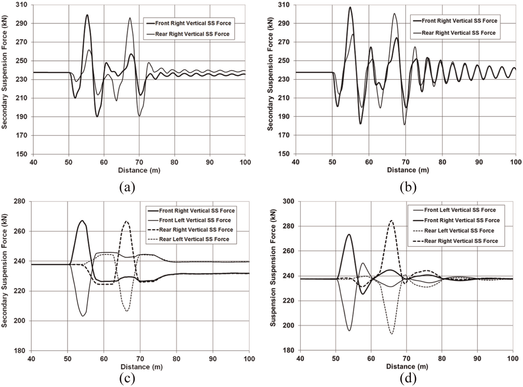
Simulated and predicted SS forces: (a) simulated SS forces due to Case 1, (b) predicted SS forces due to Case 1, (c) simulated SS forces due to Case 2 and (d) predicted SS forces due to Case 2.

Because of the same defects on both rails in Case 1, the left and right vertical SS forces are the same, so the right ones are shown in Figure 6(a) and (b). It can be also seen from these two graphs that the predicted SS forces are quite close to the simulated ones. However, in Case 2 − cross level defect – the predicted rear left and right vertical SS forces are slightly larger than the simulated ones.

WR forces

In equation (11), the external forces $\{F_w\}$ (namely, the SS forces) are known. Therefore, equation (11) can be solved through the numerical integration method – a modified Newmark-β method. Like other numerical methods, this method is also dependent upon the time step to make the solution convergence. It has been found that when the time step is selected less than $3.5\times {10}^{-5}\mathrm{s}$ , the calculated dynamic responses – WR contact forces – are stable, and the smaller time step does not change the responses significantly.

Figure 7(a)–(f) shows the WR contact forces due to Case 1 and the PS forces and the WR contact forces due to Case 2.

Figure 7.

Results due to these two irregularities: (a) simulated WR forces due to Case 1, (b) predicted WR forces due to Case 1, (c) simulated PS forces due to Case 2, (d) predicted PS forces due to Case 2, (e) simulated WR forces due to Case 2 and (f) predicted WR forces due to Case 2.

From Figure 7(a) and (b), for the type of geometry irregularity – top surface variation – the WR contact forces using the inverse modelling are comparable with the simulated ones obtained using VAMPIRE modelling. The minimum and maximum values of the WR contact forces from the simulations are 166.4 and 97.5 kN, while from the predictions, it is 163.4 and 97.0 kN, respectively, with the maximum error being 1.8%.

From Figure 7(c)–(f), for the type of geometry irregularity – cross level – the patterns of predicted results including the PS and the WR contact forces are basically consistent with the simulated ones. However, the predicted peak values for forces on the rear bogie are slightly higher than that on the front bogie (Figure 7(d) and (f)). From Figure 7(e), the two peak force values on the two wheelsets in a bogie do not happen at the same track position in the simulation, while they happen at the same track position in the inverse modelling prediction (Figure 7(f)). The reason might be that in the inverse modelling, the wagon body can only sense bogie input forces not individual wheelset forces. The minimum and maximum force values from the simulation are 103 and 141 kN on the PSs and 89 and 165.7 kN on the WR contact interfaces, while from the predictions they are 100 and 144.4 kN, and 92.5 and 163.8 kN, respectively, with the maximum error being 3.9%.

Simplified inverse modelling

In order to potentially apply the online wagon vertical inverse modelling, the model shown in Figure 1 is further simplified as a vertical model with three DoFs as shown in Figure 8.

Figure 8.

Simplified model.

In the simplified model, the following equations are assumed

$$\frac{1}{2}\left(\frac{1}{4}{M}_c\right)w^2+\frac{1}{2}\left(\frac{1}{4}{J}_{\mathrm{cy}}\right){\frac{\stackrel{·}{w}}{L_c^2}}^2=\frac{1}{2}{M}_e{\stackrel{·}{w}}^2$$

(12)

where $w$ and $\stackrel{·}{w}$ are the vertical displacement and velocity of the quarter wagon car body at a SS position. $M_c$ and $J_{\mathrm{cy}}$ are the wagon car body mass and the mass moment about the lateral direction, $L_c$ is the semi-length between bogie distance, and $M_e$ is the equivalent mass. Based on equation (12), $M_e=(1/4)(M_c+(J_{\mathrm{cy}}/L_c^2))$ , and the vertical SS force can be

$$F_{\mathrm{ss}}=M_e\times (a_m+g)=0.125\times (M_c+\frac{J_{\mathrm{cy}}}{L_c^2})\times (a_m+g)$$

(13)

where $a_m$ is the vertical acceleration of wagon car body at the position of the SS and $g$ is the acceleration due to gravity.

The track spectrums of cross level and vertical geometry irregularities similar to Class 3 specified in American Railroad, shown in Figure 9(a), are used for the simulations. At first, the dynamic responses are simulated using VAMPIRE model (Figure 3) to run on this particular track at the speed range of 10–80 km/h. Second, the accelerations on the point of car body are calculated based on the simulations and taken as the inputs into this simplified wagon inverse model for prediction calculations.

Figure 9.

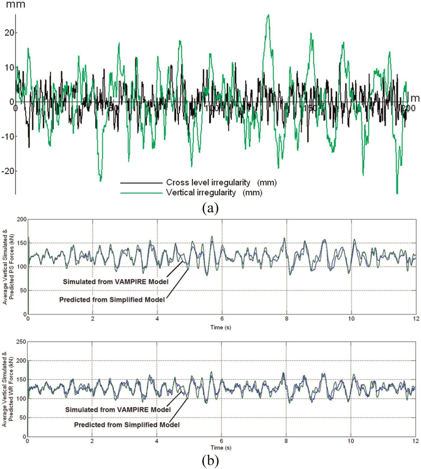
(a) Track geometry irregularity spectrums and (b) comparisons at speed of 60 km/h.

The vertical WR contact and PS forces predicted by the inverse model are compared with those from VAMPIRE simulations, shown in Figure 9(b). It has been found that the predictions by the inverse model are quite close to those simulated using the VAMPIRE model.

Table 1 lists the maximum WU rates, which are calculated by the subtractions of the minimum wheel forces from the static wheel load and then divided by the static wheel load, based on both simulation results for the speed range of 10–80 km/h.

Table 1.

Maximum wheel unloading rates (WU ≤ 0.9–1.0).

Speed (km/h)	10	20	30	40	50	60	70	80
Simulated WU (%)	7.4	17.4	21.8	26.4	34.2	29.6	52.5	93.7
Predicted WU (%)	9.1	20	26.4	27.8	33.8	31.6	48.1	87.9
Errors (%)	−23	−15	−21	−5.3	1.2	−6.7	8.3	6.1
Error average (%)	−6.9

It can be seen that for the normal operation speed of 40–80 km/h, the errors between the simulated and predicted maximum WU are reasonable.

Conclusion

A detailed two-dimensional inverse wagon modelling has been theoretically developed. The inverse wagon model can give the reasonable and useful predictions of wagon component connection forces and the WR contact forces based on the acceleration measurements on wagon components due to track geometry irregularities. In the inverse modelling, the SS forces are considered as the external forces, which are determined through the double integrations of the accelerations at the wagon car body and the SF, respectively.

The detailed inverse wagon modelling can be simplified into a few DoFs system (e.g. three DoFs in this article) for any potential online application. However, the SS forces can be directly calculated from the acceleration of wagon car body, which can significantly reduce the calculation time. It has been noticed from Table 1 that the results from the inverse model at the low speeds have some minor differences from those using a detailed VAMPIRE wagon model. However, the results at a higher speed than 40 km/h are quite agreeable, with all errors within 10%. Further improvements for the inverse wagon model and better selection of the integration and/or prediction methods and a lot of simulations on the different cases are necessary.