Sage Journals: Discover world-class research

Abstract

The axial heat transfer coefficient during flow boiling of n-hexane was measured using infrared thermography to determine the axial wall temperature in three geometrically similar annular gaps with different widths (s = 1.5 mm, s = 1 mm, s = 0.5 mm). During the design and evaluation process, the methods of statistical experimental design were applied. The following factors/parameters were varied: the heat flux $\overset{\cdot}{q} = 30 - 190 kW / m^{2}$ , the mass flux $\overset{\cdot}{m} = 30 - 700 kg / m^{2} s$ , the vapor quality $\overset{\cdot}{x} = 0.2 - 0.7$ , and the subcooled inlet temperature $T_{U} = 20 - 60 K$ . The test sections with gap widths of s = 1.5 mm and s = 1 mm had very similar heat transfer characteristics. The heat transfer coefficient increases significantly in the range of subcooled boiling, and after reaching a maximum at the transition to the saturated flow boiling, it drops almost monotonically with increasing vapor quality. With a gap width of 0.5 mm, however, the heat transfer coefficient in the range of saturated flow boiling first has a downward trend and then increases at higher vapor qualities. For each test section, two correlations between the heat transfer coefficient and the operating parameters have been created. The comparison also shows a clear trend of an increasing heat transfer coefficient with increasing heat flux for test sections s = 1.5 mm and s = 1.0 mm, but with increasing vapor quality, this trend is reversed for test section 0.5 mm.

Keywords

Flow boiling heat transfer minichannel design of experiments

Introduction

The requirements to realize high heat fluxes, to cool components at defined temperatures, and to minimize the use of hazardous or toxic media lead to simultaneous developments of increasingly smaller devices and an increased use of miniature evaporators. The resulting economic importance leads to numerous scientific studies, particularly in recent years since the work of Lazarek and Black.¹

Knowledge of the heat transfer coefficients of such equipment is of fundamental importance for the constructing engineer. The reviews of Tibiriçá and Ribatski² show that—more than 30 years later—there are different and sometimes even conflicting evidence on the effect of the parameters on the heat transfer coefficient.

The resulting need for research requires a large experimental effort to receive secured results at a maximum variation of all known factors. In addition, with this broad variance of the experimental results, the question arises whether all significant factors have already been identified and systematically investigated.

In Table 1, selected experimental works are compiled to test conditions, analysis of priorities, and the key messages. It can be seen that in many researches, the working medium, the heat flux $\overset{\cdot}{q}$ , the mass flux $\overset{\cdot}{m}$ , the subcooled inlet temperature $T_{U}$ , the vapor quality $\overset{\cdot}{x}$ , the characteristic length $l_{ch}$ , and the pressure $p$ or boiling temperature $ϑ_{S}$ were varied. The main examination focuses are on the identification and prediction of heat transfer coefficient, pressure losses, and the type of two-phase flow.

Table 1.

Flow boiling experiments with hydrocarbons and refrigerants in minichannels.

Author (year)	Fluid/channel/heating (symbols below the table)	Range of parameters	Center of research	Basic message
Agostini et al. (2008)³	R236fa, R245fa, 67 parallel □, SI, (0.223 × 0.68), L = 0.02, →↯	$\overset{\cdot}{m} = 281 - 1501 kg / m^{2} s$ $\overset{\cdot}{q} = 36 - 221 kW / m^{2}$ $p = 0.273 MPa$ ${\overset{\cdot}{x}}_{out} = 0.02 - 0.75$	α, Δp	At high $\overset{\cdot}{q}$ , α falls with increase in $\overset{\cdot}{q}$ , which is explained with intermittent dryout before CHF
Barber et al. (2009)⁴	n-pentane, □, BSG (Ta-coated), 0.4 × 4, L = 0.08, ↑, ↯↯	$\overset{\cdot}{M} = 1.13 \cdot 10^{- 5} kg / s$ $\overset{\cdot}{q} = 4.26 kW / m^{2}$	Instabilities in α, Δp, T_W , flow pattern	Assumes that steam rebounds are responsible for temperature and pressure fluctuations
Callizo (2010)⁵	R134a, R22, ○, ES, L ≈ 0.22 m, ↑, ↯↯ d = (1.7; 1.224; 0.826; 0.64), s = (0.25; 0.38; 0.187; 0.13), ○, quartz GL (In-Sn-coated), d = 1.332, s = 2.384, L = 0.24, ↑, ↯↯	$\overset{\cdot}{m} = 100 - 700 kg / m^{2} s$ $\overset{\cdot}{q} = 1 - 68.7 kW / m^{2}$ $T_{U} = 3 - 15 K$ $p_{in} = 0.77 - 1.02 MPa$ ${\overset{\cdot}{x}}_{out} = - 0.17 - 0.97$	α, Δp, CHF, comparison of correlations, flow pattern	At $\overset{\cdot}{x} \leq 0$ , α increases with increasing T_U, p, and reducing d. From $\overset{\cdot}{x} \geq 0.5$ , intermittent dryout, α falls, influence of $\overset{\cdot}{q}$ decreases
Cavallini et al. (2007)⁶	R134a, ○, Cu, d = 0.96, s = 3.52, L = 0.24, →, water	$\overset{\cdot}{m} = 300 - 600 kg / m^{2} s$ $\overset{\cdot}{q} = 60 - 110 kW / m^{2}$ ${\overset{\cdot}{x}}_{dryout} \leq 0.8$	Dryout	Low dependence of $\overset{\cdot}{m}$ and $\overset{\cdot}{q}$ found
Celata et al. (2011)⁷	FC-72, ○, BSG, d = 0.48, s = 0.158, L = 0.073, →, glykol	$\overset{\cdot}{m} = 50 - 3000 kg / m^{2} s$ $\overset{\cdot}{q} \leq 65 kW / m^{2}$ ${\overset{\cdot}{x}}_{out} \leq 0.8$	α, flow pattern, instabilities on boiling	Nucleate boiling mainly at negative $\overset{\cdot}{x}$ . Influence of $\overset{\cdot}{m}$ and $\overset{\cdot}{x}$ on α at higher $\overset{\cdot}{x}$
Choi et al. (2009)⁸	Propane, ○, ES, d = 1.5; 3, L = 1; 2, →, ↯↯	$\overset{\cdot}{m} = 50 - 400 kg / m^{2} s$ $\overset{\cdot}{q} = 5 - 20 kW / m^{2}$ ϑ_S = 0 °C; 5 °C; 10 °C ${\overset{\cdot}{x}}_{out} \leq 1$	α, Δp, comparison of correlations, new correlation	α shows dependence on $\overset{\cdot}{m}$ , $\overset{\cdot}{q}$ , ϑ_S , and the tube diameter
Copetti et al. (2013)⁹	Isobutene, ○, ES, L = 0.185, ○, GL, L = 0.158, d = 2.6, →, ↯↯	$\overset{\cdot}{m} = 240 - 440 kg / m^{2} s$ $\overset{\cdot}{q} = 44 - 95 kW / m^{2}$ ϑ_S = 22 °C ${\overset{\cdot}{x}}_{out} \leq 0.7$	α, Δp, flow pattern, comparison of correlations	In highest values of $\overset{\cdot}{q}$ , $α \neq f (\overset{\cdot}{m})$ , $\overset{\cdot}{m}$ and $\overset{\cdot}{x}$ have significant effect on Δp
Díaz et al. (2008)¹⁰	n-hexane, n-oktane, ⊚, ES-ES, d_i,a = 5, d_a,i = 6, ⊚, ES-BSG, d_i,a = 6, d_a,i = 7, s = 0.5, L = 0.3, ↑, ↯↯	$\overset{\cdot}{m} = 50 - 300 kg / m^{2} s$ $\overset{\cdot}{q} \leq 250 kW / m^{2}$ p_out = 0.1 MPa ${\overset{\cdot}{x}}_{out} \leq 0.75$	α, flow pattern	Annular flow with intermittent dryouts of wall film destruction as a result of observed liquid-vapor waves
Harirchian and Garimella (2012)¹¹	FC-77, five different multi-channels 2-60×□, SI, (5.85-0.1 × 0.4), →, ↯	$\overset{\cdot}{m} = 225 - 1461 kg / m^{2} s$ $\overset{\cdot}{q} \leq 380 kW / m^{2}$ p_out = 0.1 MPa ${\overset{\cdot}{x}}_{out} \leq 1$	α, Δp, comparison of correlations, new correlation	Flow pattern based on correlations provide higher accuracy
Hozejowska et al. (2009)¹²	R123, R11, □, ES, (0.7; 1; 1.5; 2 × 20; 40), L = 0.36, s = 0.1, ↑, ↯↯	$\overset{\cdot}{m} = 412 kg / m^{2} s$ $\overset{\cdot}{q} = 82 - 886 kW / m^{2}$ p_in = 0.19 MPa T_U = 36 K	α, ONB, hysteresis	Boiling front is accompanied by a decrease in local wall temperature
Maqbool et al. (2013)¹³	Propane, ○, ES, GL, d = 1.7, L = 0.245, ↑, ↯↯	$\overset{\cdot}{m} = 100 - 500 kg / m^{2} s$ $\overset{\cdot}{q} = 5 - 280 kW / m^{2}$ ϑ_S = 23 °C–43 °C $\overset{\cdot}{x} = 0 - 1$	α, Δp, dryout, flow pattern, comparison of correlations	α increases with increasing $\overset{\cdot}{q}$ and ϑ_S . Δp rises with increasing $\overset{\cdot}{q}$ , $\overset{\cdot}{m}$ , $\overset{\cdot}{x}$ , and decreasing ϑ_S . Correlations inexact in range of dryout
Oh et al. (2011)¹⁴	R22, R134a, R410A, propane, CO₂, ○, ES, L = (0.33; 1; 1.5; 2; 3), d = (0.5; 1.5; 3), →, ↯↯	$\overset{\cdot}{m} = 100 - 1600 kg / m^{2} s$ $\overset{\cdot}{q} = 5 - 40 kW / m^{2}$ ϑ_S = 0 °C–15 °C $\overset{\cdot}{x} \leq 1$	α, comparison of correlations, new correlation	At low $\overset{\cdot}{x}$ , $α = f (\overset{\cdot}{q})$ and at higher $\overset{\cdot}{x}$ , $α = f (\overset{\cdot}{m})$ , α increases with increasing ϑ_S and small d
Ong and Thome (2009)¹⁵	R134a, R236fa, R245fa, ○, ES, BSG, d = 1.03, L = 0.18, →, ↯↯	$\overset{\cdot}{m} = 200 - 1600 kg / m^{2} s$ $\overset{\cdot}{q} = 2.3 - 250 kW / m^{2}$ ϑ_S = 31 °C T_U = 2–9 K, $\overset{\cdot}{x} = 0 - 1$	α, flow pattern	α increases with increasing $\overset{\cdot}{q}$ over a wide range of $\overset{\cdot}{x}$ at low $\overset{\cdot}{m}$ , α decreases in the transition from bubble to plug flow
Ozer et al. (2010)¹⁶	R11, Novec 649, □, ES, GL, (1.2 × 23), s = 0.075, L = 0.357, →, ↯↯	$\overset{\cdot}{m} = 52 kg / m^{2} s$ $\overset{\cdot}{q} = 342 - 58 kW / m^{2}$ p = 0.24–0.26 MPa T_U = 29.5–32.6 K	α, flow pattern	At the boiling front, α is dominated by already deformed slide bubbles and not uniformly distributed bubble nuclei
Pamitran et al. (2011)¹⁷	C₃ H₈, NH₃, CO₂, ○, ES, d = (1.5; 3), L = 2, →, ↯↯	$\overset{\cdot}{m} = 50 - 600 kg / m^{2} s$ $\overset{\cdot}{q} = 5 - 70 kW / m^{2}$ ϑ_S = 0 °C–10 °C $\overset{\cdot}{x} = 0 - 1$	α	Small $\overset{\cdot}{x}$ : clear influence of $\overset{\cdot}{q}$ but no influence of $\overset{\cdot}{m}$ and $\overset{\cdot}{x}$ . High $\overset{\cdot}{m}$ : α increase for less $\overset{\cdot}{x}$ . Medium $\overset{\cdot}{x}$ : α increase with increasing $\overset{\cdot}{m}$ , $\overset{\cdot}{x}$
Piasecka (2013)¹⁸	FC-72, □, ES, GL, (1 × 60), s = 0.1, L = 0.36, →, ↑, ↯↯	$\overset{\cdot}{m} = 137 - 285 kg / m^{2} s$ $\overset{\cdot}{q} = 115 - 347 kW / m^{2}$ p = 0.12–0.125 MPa T_U = 30–42 K	Δp, α, φ, flow pattern, flow pattern maps	α at the boiling front rises first, then drops significantly. Good agreement of Δp_exp with a theoretical model in ↑ channel
Rahim et al. (2011)¹⁹	R134a, R245fa, ○, ES, GL, d = (0.709; 0.509), L = 0.11, →, ↯↯	$\overset{\cdot}{m} = 210 - 2094 kg / m^{2} s$ $\overset{\cdot}{q} = 3 - 415 kW / m^{2}$ ϑ_S = 26 °C; 30 °C; 35 °C $\overset{\cdot}{x} = 0 - 0.95$	Flow pattern, flow pattern maps	Rarely bubble flow, slug, and annular flow dominate. Good agreement with the model of Ullmann and Brauner²⁰
Revellin et al. (2008)²¹	R134a, ○, ES, GL, d = (0.709; 0.509), L = 0.11, →, ↯↯	$\overset{\cdot}{m} = 200 - 1500 kg / m^{2} s$ $\overset{\cdot}{q} = 65 - 318 kW / m^{2}$ ϑ_S = 26 °C–35 °C T_U = 2–5 K	Flow pattern, bubble collisions	The prediction of bubble collisions favor the creation of theoretically based flow pattern maps
Shiferaw et al. (2009)²²	R134a, ○, ES, BSG, d = 1.1, s = 0.247, L = 0.15, ↑, ↯↯	$\overset{\cdot}{m} = 100 - 600 kg / m^{2} s$ $\overset{\cdot}{q} = 16.7 - 170 kW / m^{2}$ p = 0.6–1.2 MPa $\overset{\cdot}{x} \leq 0.9$	α, flow pattern, comparison of 3-zone model	At $\overset{\cdot}{x} \leq 0.5$ , α increases with increasing $\overset{\cdot}{q}$ and p. Then α falls with higher $\overset{\cdot}{x}$ , which was explained by partial dryout
Wen and Ho (2005)²³	Propane, butane, propane/butane (55 Wt%), ○, Cu, d = 2.46, s = 0.36, →, L = 3.85, water	$\overset{\cdot}{m} = 250 - 500 kg / m^{2} s$ $\overset{\cdot}{q} = 5 - 21 kW / m^{2}$ p_out = 0.1 MPa ${\overset{\cdot}{x}}_{out} \leq 0.86$	α, Δp, comparison α_exp with α_Mod , new correlation	Heat transfer improves with increasing $\overset{\cdot}{m}$ and $\overset{\cdot}{q}$ values
Yang et al. (2013)²⁴	Kerosin, ○, ES d = 2, s = 0.5, L = 0.14–0.42, ↑, ↯↯	$\overset{\cdot}{m} = 213 - 640 kg / m^{2} s$ $\overset{\cdot}{q} = 220 - 1100 kW / m^{2}$ p_in = 2–2.7 MPa ϑ_in = 25 °C	α, Δp, flow pattern	Heated length has important influence on the process

ES: stainless steel; BSG: borosilicate glass; GL: glass; SI: silicone ;CHF: critical heat flux; ONB: onset of nucleate boiling; →: horizontal; ↑: vertical; □: rectangular channel; ○: tube; ⊚: annular gap; ↯↯: direct electric heating; ↯: electric heating; tube diameter d, respectively, channel width and height in mm, channel length L in m, and wall thickness s in mm.

Methods

Experimental setup

The test rig is designed for heat transfer experiments and visualizations of the two-phase flow.²⁵ Figure 1 shows the schematic structure of the test stand in the case of the determination of the heat transfer coefficient. The working fluid is conveyed by means of a variable speed micro-dosing pump from an open to the atmosphere reservoir to a Coriolis mass flow meter. The subcooled inlet temperature is then adjusted in a heat exchanger before the medium enters the electrically directly heated test section, as shown in Figure 2. The partially evaporated medium is liquefied and subcooled in a condenser.

Figure 1.

Experimental setup.

Figure 2.

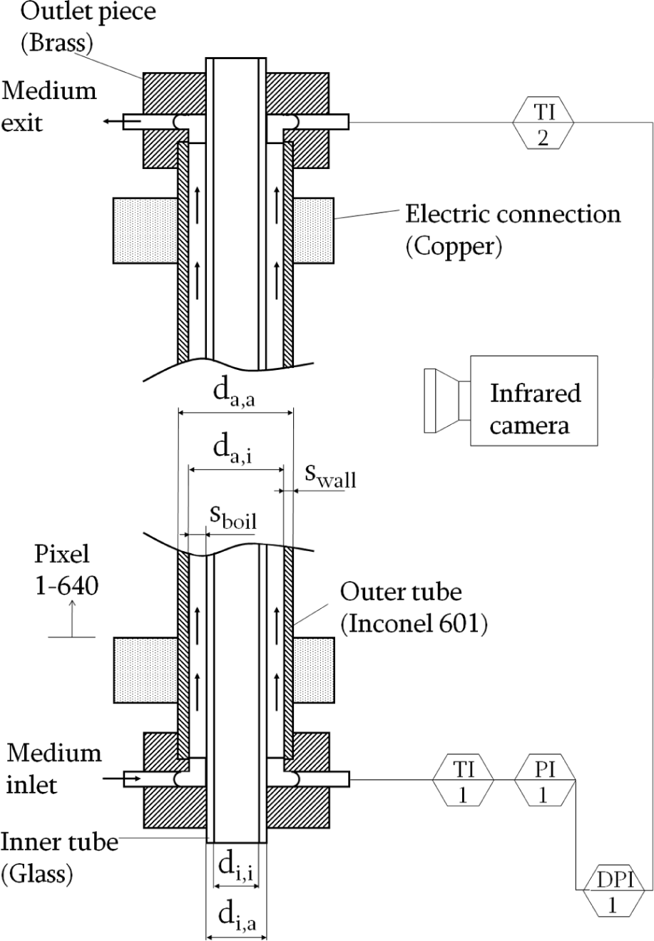
Test section.

At the inlet and outlet of the test section, the temperature is measured by thermocouples and the differential pressure is determined. Together with the measurement of the absolute pressure on the inlet, the pressure-dependent saturation temperature is determined. The analysis of the axial wall temperature profile is realized by an infrared (IR) camera. The experimental evaluation is implemented in LabVIEW and provides a superior in-process analysis of the axial heat transfer coefficient.

Test sections

The test sections are designed as annular gaps. The outer metallic tube is electrically heated directly and made of Inconel 601 which is coated with a thin layer of special black lacquer to provide large values of emissivity. Inconel 601 has a low dependence of the electrical resistivity from the wall temperature and high thermal resistance, so that the evaporation experiments can be carried out approximately at the boundary condition $\overset{\cdot}{q} = constant$ . Due to reasons of electrical insulation, and thus, the unique electrical heating, the inner tube is made of borosilicate glass. The dimensions of the test sections are given in Table 2.

Table 2.

Dimensions of the test sections with variation of the characteristic length.

s_boil (µm)	d_i,i (mm)	d_i,a (mm)	d_a,i (mm)	d_a,a (mm)	d_a,i /d_i,a	L (mm)
500	1.2	4	5	6	1.25	300
1000	3	8	10	11	1.25	300
1500	8.4	12	15	16	1.25	300

The geometric similarity of the different test sections is ensured by the constancy of the diameter ratio d_a,i /d_i,a . The heating wall is s_Wall = 0.5 mm thick in all test sections to ensure comparability of the boiling processes.

The heat losses ${\overset{\cdot}{q}}_{loss}$ by convection and radiation were measured at all test sections. For this purpose, the annular gap was dry, that is filled with air, and the duct temperature was determined by thermocouples in the inner tube. Due to an additional heating of the electrical connections, the influences of cross heat conduction were minimized. By means of the values of the direct current (DC) power sources, the heat loss could be calibrated as a function of the metallic outer wall temperature. It has to be noted that the axial temperature profile during the calibration deviates slightly from that in the experiment due to the subcooled boiling. In the range of saturation boiling, this deviation is negligible.

The same configuration was used to allow the IR thermographic determination of the metal outside wall temperature, with the difference that the test section was positioned horizontally here to reach a possible homogeneous temperature in the channel. Using the measured inner wall temperature and the known heat losses, it is then possible to determine the metallic wall outside temperature by solving the stationary one-dimensional heat conduction problem with uniformly distributed source. With simultaneous IR thermographic examination, the calculated metal outside wall temperature can then assign a corresponding signal of the IR camera and thus eliminates the inaccuracies resulting from the coating layer.

To verify the measurement setup, single-phase experiments were carried out, and the results of the heat transfer coefficient were compared with numerical solutions from the literature.²⁶ In order to perform these tests in the parameter ranges which are relevant to the two-phase experiments, n-decane is used as experimental medium. This working medium provides similar physical and thermal properties at a higher boiling temperature. However, the verification measurements showed over a wide range of parameter deviations of less than 10% which increased with decreasing characteristic lengths and heat fluxes, but not above 30%.

All essential calculations are realized online, which means “in-process” during the experiment, resulting in significant advantages compared to the post-process analysis. Among other things, it is possible to effectively study the dynamics of the boiling process after parameter changes, the interaction between the parameters, and their influence on the heat transfer. It also improves the unit safety and minimizes the evaluation costs.

Data reduction

The local heat transfer coefficient α(z) is defined through equation (1)

α (z) = \frac{\overset{\cdot}{q} (z)}{T_{W, i} (z) - T_{fl} (z)}

(1)

The heat flux $\overset{\cdot}{q} (z)$ therein, equation (2)

\overset{\cdot}{q} (z) = \frac{ρ_{el} (z) I^{2}}{\frac{π^{2}}{4} (d_{a, a}^{2} - d_{a, i}^{2}) \cdot d_{a, i}} - \frac{d_{a, a}}{d_{a, i}} {\overset{\cdot}{q}}_{loss} (z)

(2)

is aside from the low temperature dependence of the electric resistivity ρ_el (z) and the axial changes in heat losses ${\overset{\cdot}{q}}_{loss} (z)$ approximately constant.

By solving the stationary one-dimensional heat conduction problem with source using the Fourier’s equation and knowing the metallic wall outside temperature T_Wa,m (z) and the heat losses to the environment, the inside wall temperature T_W,i (z) contained in equation (1) is determined with equation (3)

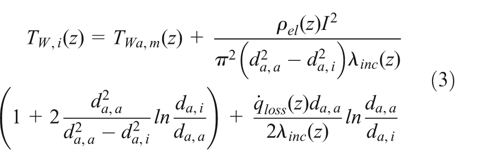
\begin{matrix} T_{W, i} (z) = T_{Wa, m} (z) + \frac{ρ_{el} (z) I^{2}}{π^{2} (d_{a, a}^{2} - d_{a, i}^{2}) λ_{inc} (z)} \\ (1 + 2 \frac{d_{a, a}^{2}}{d_{a, a}^{2} - d_{a, i}^{2}} \ln \frac{d_{a, i}}{d_{a, a}}) + \frac{{\overset{\cdot}{q}}_{loss} (z) d_{a, a}}{2 λ_{inc} (z)} \ln \frac{d_{a, a}}{d_{a, i}} \end{matrix}

(3)

The thermal conductivity λ_inc (z) is determined depending on the channel temperature. To calculate the axial fluid temperature T_fl (z) in single-phase and in the subcooled boiling area, the caloric mean temperature ${\bar{T}}_{fl}$ is used in equation (4)

\begin{matrix} {\bar{T}}_{fl} (z = 0) = T_{Fl, in} \\ {\bar{T}}_{fl} (z + Δ z) = {\bar{T}}_{fl} (z) + \frac{4 \overset{\cdot}{q} (z) \cdot Δ z}{\overset{\cdot}{m} \cdot c_{fl} (z)} \frac{d_{a, i}}{(d_{a, a}^{2} - d_{a, i}^{2})} \end{matrix}

(4)

contained therein, the specific heat capacity $c_{fl} ({\bar{T}}_{fl} (z))$ is determined iteratively.

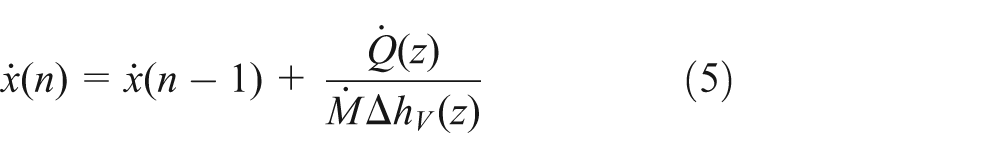
When the caloric fluid mean temperature reaches the pressure-dependent boiling temperature ${\bar{T}}_{fl} (z) = T_{S} (p)$ , the local heat transfer coefficient is calculated in subsequent axial course using the pressure-dependent boiling temperature, wherein the axial pressure curve of linearization of the inlet and outlet pressure follows.

As a dimensionless coordinate, the theoretical vapor quality $\overset{\cdot}{x}$ is used. In this case, the theoretical vapor quality $\overset{\cdot}{x} = 0$ , by definition, is assigned with the axial position where ${\bar{T}}_{fl} (z) = T_{S} (p (z))$ . The other $\overset{\cdot}{x}$ curve can be calculated using equation (5)

\overset{\cdot}{x} (n) = \overset{\cdot}{x} (n - 1) + \frac{\overset{\cdot}{Q} (z)}{\overset{\cdot}{M} Δ h_{V} (z)}

(5)

How Díaz and Schmidt²⁷ showed a two-phase flow can be registered even before $\overset{\cdot}{x} = 0$ . In order to make the analysis of the heat transfer coefficient in the range of subcooled boiling, a negative vapor quality (equation (6)) was defined

\overset{\cdot}{x} (n) = \overset{\cdot}{x} (n + 1) - \frac{\overset{\cdot}{Q} (z)}{\overset{\cdot}{M} Δ h_{V} (z)}

(6)

The enthalpy of evaporation Δh_V (z) herein is determined as a function of the local pressure-dependent boiling temperature.

In excerpts, the course of the calculated temperatures and the resulting heat transfer coefficient is shown in Figure 3 for the gap width 0.5 mm and in Figure 4 for the gap width 1.5 mm. It is observed that, due to the nearly constant heat flux, the heat transfer coefficient increases with decreasing difference between the fluid temperature T_fl (z) and the inner wall temperature T_W,i (z).

Figure 3.

Temperatures and heat transfer coefficient as a function of vapor quality: s = 0.5 mm; $\overset{\cdot}{m} = 299 kg / m^{2} s$ ; $\overset{\cdot}{q} = 120 kW / m^{2}$ ; T_U = 20 K; P_in = 0.21 MPa.

Figure 4.

Temperatures and heat transfer coefficient as a function of vapor quality: s = 1.5 mm; $\overset{\cdot}{m} = 59 kg / m^{2} s$ ; $\overset{\cdot}{q} = 65 kW / m^{2}$ ; T_U = 40 K; P_in = 0.19 MPa.

The error estimate is subject to the rules of error propagation law. For analysis at the single-phase preheating and the subcooled boiling, the estimation is done with equation (7)

\begin{matrix} Δ α_{abs}^{2} (\overset{\cdot}{x} < 0) = {(\frac{δ α}{δ I})}^{2} Δ I^{2} + {(\frac{δ α}{δ \overset{\cdot}{M}})}^{2} Δ {\overset{\cdot}{M}}^{2} \\ + {(\frac{δ α}{δ T_{Wa, m}})}^{2} Δ T_{Wa, m}^{2} + \dots \\ \dots + {(\frac{δ α}{δ T_{Fl, in}})}^{2} Δ T_{Fl, in}^{2} + {(\frac{δ α}{δ d_{a, a}})}^{2} Δ d_{a, a}^{2} + {(\frac{δ α}{δ d_{a, i}})}^{2} Δ d_{a, i}^{2} \end{matrix}

(7)

and equation (8) is used for the area of saturation boiling

\begin{matrix} Δ α_{abs}^{2} (\overset{\cdot}{x} \geq 0) = {(\frac{δ α}{δ I})}^{2} Δ I^{2} + {(\frac{δ α}{δ p})}^{2} Δ p^{2} \\ + {(\frac{δ α}{δ T_{Wa, m}})}^{2} Δ T_{Wa, m}^{2} + \dots \\ \dots + {(\frac{δ α}{δ d_{a, a}})}^{2} Δ d_{a, a}^{2} + {(\frac{δ α}{δ d_{a, i}})}^{2} Δ d_{a, i}^{2} \end{matrix}

(8)

The uncertainty in the electrical current measurement is ΔI = 0.4 A and in the mass flux $\overset{\cdot}{M}$ determination 0.15% of the measurement value. The error in the outer wall temperature measurement caused by uncertainty in the emissivity and in the wall thickness of the coated metallic wall is ΔT_Wa ,_m = 0.4 K, and the pressure measurement uncertainty which influences the boiling temperature accuracy is Δp = 560 Pa. ΔT_Fl ,_in = 0.1 K is the error of the thermocouple with which the fluid inlet temperature is determined. Δd_a ,_a = 0.01 mm and Δd_a ,_i = 0.06 mm are the geometric inaccuracies of the outer and the inner diameters. The analysis of the experimental uncertainties leads to an average error in the heat transfer coefficient Δα_abs within the preheating and subcooled boiling range of 8%−30% and in the saturated boiling range of below 10%. Not included are the errors resulting from the concentricity of both tubes.

This study aims to provide a better understanding of two-phase flow and boiling characteristics during the transition from conventional to miniaturized channels. With regard to the problem of fuel evaporation, n-hexane is used as a working medium.

There are problems regarding the parameter settings of which one results from the complex boiling process. In case the heat flux is changed when setting a new test point, the pressure curve, the boiling pressure-dependent subcooled inlet temperature, and the mass flux change at constant pump speed due to the changing boiling process. With regard to these conditions and planning experiments according to the classic principle “one factor at a time”, the mass flux and the subcooled inlet temperature need to be adjusted. In addition to these two parameters influencing each other, a change of measurement result (heat transfer coefficient) cannot be clearly assigned to a change of heat flux, as the boiling pressure also changes. The method of “one factor at a time” is difficult to realize, as the pressure curve, which is a parameter with influence on the boiling process and the two-phase flow, is changed with each parameter change. To better meet these requirements of the complex boiling process, this project uses the method developed by Fisher²⁸“Design of Experiments” (DoE).

DoE

Even after intensive research, no publications were found to apply these methods to the study of the flow boiling. The advantages of this approach are, among others, minimal experimental effort and associated costs as well as secure statements that can be made under consistent implementation.

Critical to the quality of the test results are the detailed description of the system to be examined and the influencing parameters (Figure 5) which can be distinguished as parameters that can be selectively altered and those that cannot be specifically altered. With this parameter constellation, system results are obtained.

Figure 5.

Description of the system.

For this investigation, the heat and mass flux and the subcooled inlet temperature at evaporator systems with three different gap widths were varied systematically. Parameters are not specifically varied for the inlet pressure and the pressure drop across the channel and other unknown parameters. The results of these parameters applied to the system are the set system responses such as the heat transfer coefficient and the vapor quality.

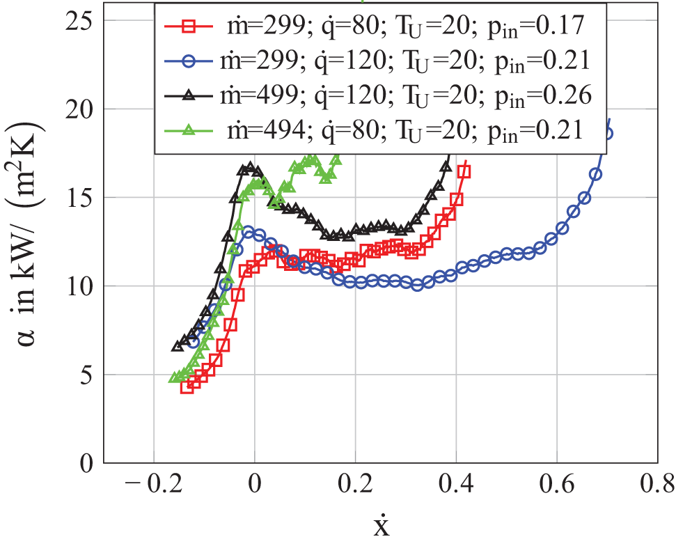
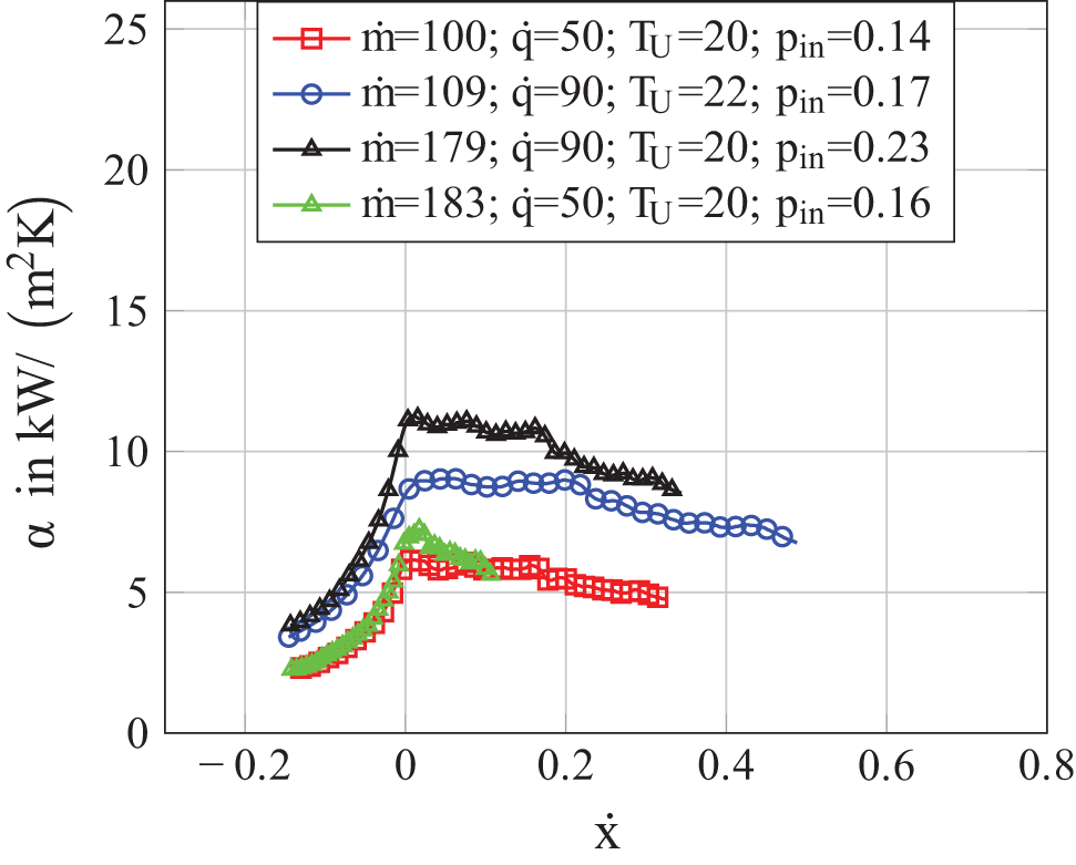
As shown in Figures 6 –8, there is a great local diversity of these system responses. To limit this diversity within first evaluation, Boye²⁵ gives a definition of the mean heat transfer coefficients for the ranges of single-phase preheating and subcooled boiling $(\overset{\cdot}{x} < 0)$ , transition from subcooled to saturated boiling $(\overset{\cdot}{x} \approx 0)$ , and saturated boiling $(\overset{\cdot}{x} > 0)$ .

Figure 6.

Heat transfer coefficient as a function of vapor quality: s = 0.5 mm; $\overset{\cdot}{m} (kg / m^{2} s)$ ; $\overset{\cdot}{q} (kW / m^{2})$ ; T_U (K); p_in (MPa).

Figure 7.

Heat transfer coefficient as a function of vapor quality: s = 1.0 mm; $\overset{\cdot}{m} (kg / m^{2} s)$ ; $\overset{\cdot}{q} (kW / m^{2})$ ; T_U (K); p_in (MPa).

Figure 8.

Heat transfer coefficient as a function of vapor quality: s = 1.5 mm; $\overset{\cdot}{m} (kg / m^{2} s)$ ; $\overset{\cdot}{q} (kW / m^{2})$ ; T_U (K); p_in (MPa).

The vapor quality is already fully described by the input variables (equations (6) and (5)); therefore, the model for this system response is already known. Since the vapor quality is an important parameter for the characterization of the two-phase flow, it should be considered when modeling the heat transfer coefficient. Kleppmann²⁹ proposes to model the system response as an input variable if this is advantageous to describe the system. In the following experimental evaluation, the channel length is divided into 60 equidistant areas. Each area has an axial dimension of 10 IR pixels corresponding to around 5 mm of the channel length. For each of these sectors, arithmetically averaged vapor qualities and heat transfer coefficients are calculated as an input variable of the system and as the system response.

The example of a local system response in Figure 6 for the gap width s = 0.5 mm shows a significant increase in the local heat transfer coefficient in the range of subcooled boiling. At the beginning of saturated boiling, it provides a local maximum with a subsequent decrease in the local heat transfer coefficient which then increases again at higher vapor qualities.

Since discontinuity and local extremum are difficult to model, scopes $\overset{\cdot}{x} < 0$ and $\overset{\cdot}{x} > 0$ are defined where no discontinuity occurs to improve the prediction accuracy. Thus, for each gap width, two correlations were determined (see Table 4)

\begin{matrix} α = & c_{0} + c_{1} \overset{\cdot}{m} + c_{2} \overset{\cdot}{q} + c_{3} T_{U} + c_{4} \overset{\cdot}{x} + c_{5} \overset{\cdot}{m} \overset{\cdot}{q} + c_{6} \overset{\cdot}{m} T_{U} + \dots \\ \dots + c_{7} \overset{\cdot}{m} \overset{\cdot}{x} + c_{8} \overset{\cdot}{q} T_{U} + c_{9} \overset{\cdot}{q} \overset{\cdot}{x} + c_{10} T_{U} \overset{\cdot}{x} + \dots \\ \dots + c_{11} {\overset{\cdot}{m}}^{2} + c_{12} {\overset{\cdot}{q}}^{2} + c_{13} T_{U}^{2} + c_{14} {\overset{\cdot}{x}}^{2} \end{matrix}

(9)

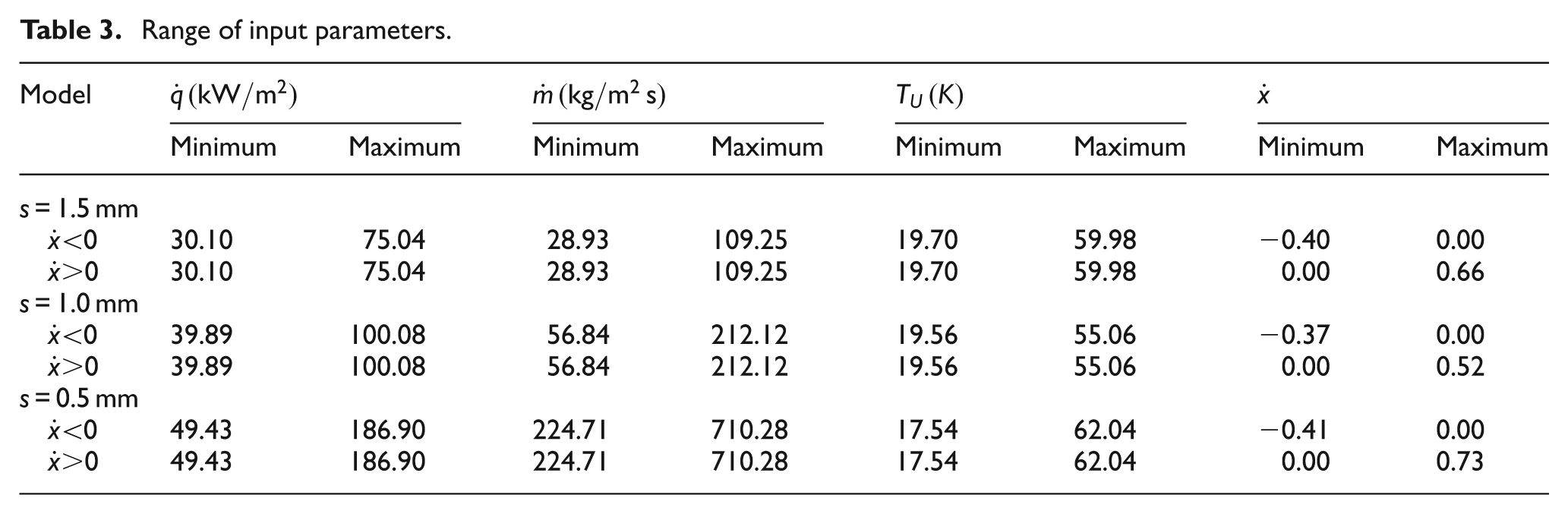
These empirical models (equation (9)) have been developed as a function of normalized operating parameters; thus, the minimum parameter value is assigned with −1 and the maximum parameter value is assigned with +1 (Table 3). The comparisons of the results of these correlations show qualitative and quantitative differences regarding the influences of parameter changes as a function of the gap widths.

Table 3.

Range of input parameters.

Model	$\overset{\cdot}{q} (kW / m^{2})$		$\overset{\cdot}{m} (kg / m^{2} s)$		$T_{U} (K)$		$\overset{\cdot}{x}$
	Minimum	Maximum	Minimum	Maximum	Minimum	Maximum	Minimum	Maximum
s = 1.5 mm
$\overset{\cdot}{x} < 0$	30.10	75.04	28.93	109.25	19.70	59.98	−0.40	0.00
$\overset{\cdot}{x} > 0$	30.10	75.04	28.93	109.25	19.70	59.98	0.00	0.66
s = 1.0 mm
$\overset{\cdot}{x} < 0$	39.89	100.08	56.84	212.12	19.56	55.06	−0.37	0.00
$\overset{\cdot}{x} > 0$	39.89	100.08	56.84	212.12	19.56	55.06	0.00	0.52
s = 0.5 mm
$\overset{\cdot}{x} < 0$	49.43	186.90	224.71	710.28	17.54	62.04	−0.41	0.00
$\overset{\cdot}{x} > 0$	49.43	186.90	224.71	710.28	17.54	62.04	0.00	0.73

Results and discussion

The main objective of this work is the study of the flow boiling heat transfer characteristics under stable operating conditions with variation of geometric and operating parameters. The relevant experimental analysis encounters objective difficulties in necessary overlap of the parameter ranges on variation of the characteristic length. According to the energy balance equation (10)

\overset{\cdot}{m} = \overset{\cdot}{q} \frac{4 Δ z}{(d_{a, i} - d_{i, a}^{2} / d_{a, i}) Δ \overset{\cdot}{x} Δ h_{V}} = \overset{\cdot}{q} \cdot f (d) \frac{4 Δ z}{Δ \overset{\cdot}{x} Δ h_{V}}

(10)

for a given medium, the function $f (d) = 1 / (d_{a, i} - d_{i, a}^{2} / d_{a, i})$ defines the size of the relation $\overset{\cdot}{m} / \overset{\cdot}{q}$ to achieve a certain vapor quality by the different test sections (Figure 9). This means, for example, for a given heat flux, the realistic mass flux decreases with increasing characteristic length. Together with the limitations of the micro-dosing pump, the DC power source, the preheater and condenser, and the range of input parameters for each test sections are arised in Table 3.

Figure 9.

Influence of the diameter on the operating parameters.

Basically, with regard to the diameter dependence of the heat transfer coefficient in the two-phase flow, it is to expect that this is decreasing when the characteristic length increases. This principle can be confirmed in consideration of Figures 6 –8. The trend of the heat transfer coefficients shown for all three test sections are rising α values in the range of subcooled boiling, wherein the level of heat transfer coefficients with smaller gap width and higher heat flux increases significantly and no dependence from the mass flux is noticed. The transition from subcooled flow boiling to saturated flow boiling is characterized by a local maximum in the heat transfer coefficient. Following, the profile of the heat transfer coefficient shows a significant differentiation depending on the characteristic length. For the gap widths of s = 1.0 mm and s = 1.5 mm (Figures 7 and 8), a monotonically decreasing heat transfer coefficient for all parameter constellations can be noticed. 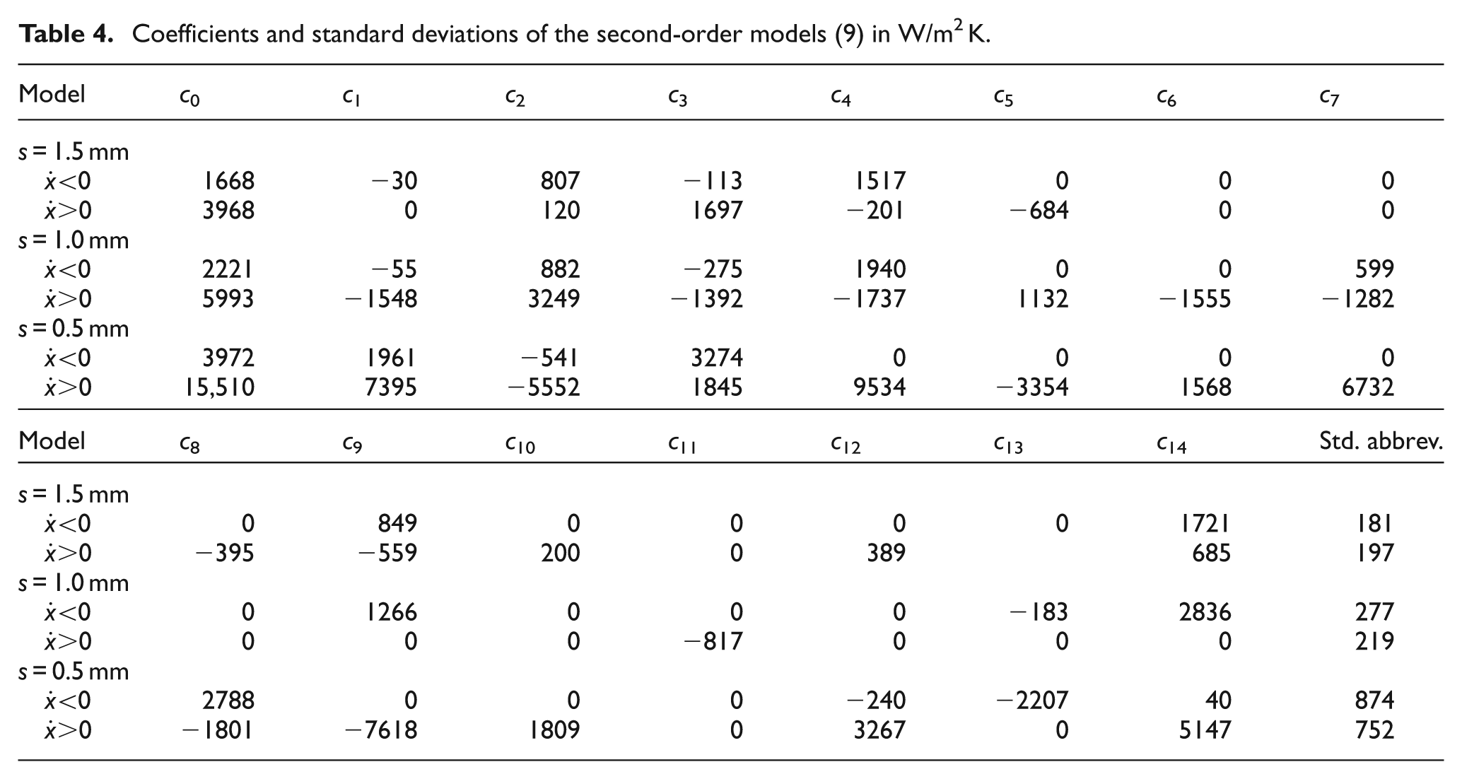Here too, as in the area of subcooled boiling, a low $\overset{\cdot}{m}$ dependence and higher α values with increasing heat flux were registered. By reducing the gap width, the influence of $\overset{\cdot}{m}$ increases significantly, as shown in Figure 6, and the influence of the heat flux shows an opposite trend toward lower heat transfer coefficient with increasing heat flux.

A more detailed insight into the influence of the operating and above all also geometrical parameters can be obtained by modeling the heat transfer coefficient, as given in equation (9). The coefficients contained therein are given in Table 4. As already explained in the “DoE” section, two correlations were determined for each test section, shown in Figure 10(a)–(d) for $\overset{\cdot}{x} < 0$ , as well as for $\overset{\cdot}{x} > 0$ in Figures 10(e), (f), and 11.

Table 4.

Coefficients and standard deviations of the second-order models (9) in W/m² K.

Model	c ₀	c ₁	c ₂	c ₃	c ₄	c ₅	c ₆	c ₇
s = 1.5 mm
$\overset{\cdot}{x} < 0$	1668	−30	807	−113	1517	0	0	0
$\overset{\cdot}{x} > 0$	3968	0	120	1697	−201	−684	0	0
s = 1.0 mm
$\overset{\cdot}{x} < 0$	2221	−55	882	−275	1940	0	0	599
$\overset{\cdot}{x} > 0$	5993	−1548	3249	−1392	−1737	1132	−1555	−1282
s = 0.5 mm
$\overset{\cdot}{x} < 0$	3972	1961	−541	3274	0	0	0	0
$\overset{\cdot}{x} > 0$	15,510	7395	−5552	1845	9534	−3354	1568	6732
Model	c ₈	c ₉	c ₁₀	c ₁₁	c ₁₂	c ₁₃	c ₁₄	Std. abbrev.
s = 1.5 mm
$\overset{\cdot}{x} < 0$	0	849	0	0	0	0	1721	181
$\overset{\cdot}{x} > 0$	−395	−559	200	0	389		685	197
s = 1.0 mm
$\overset{\cdot}{x} < 0$	0	1266	0	0	0	−183	2836	277
$\overset{\cdot}{x} > 0$	0	0	0	−817	0	0	0	219
s = 0.5 mm
$\overset{\cdot}{x} < 0$	2788	0	0	0	−240	−2207	40	874
$\overset{\cdot}{x} > 0$	−1801	−7618	1809	0	3267	0	5147	752

Figure 10.

Results of the correlations for $\overset{\cdot}{x} \leq 0$ : (a) T_U = 20 K, $\overset{\cdot}{x} = - 0.1$ ; (b) T_U = 40 K, $\overset{\cdot}{x} = - 0.1$ ; (c) T_U = 20 K, $\overset{\cdot}{x} = 0$ , using the model $\overset{\cdot}{x} < 0$ ; (d) T_U = 40 K, $\overset{\cdot}{x} = 0$ , using the model $\overset{\cdot}{x} < 0$ ; (e) T_U = 20 K, $\overset{\cdot}{x} = 0$ , using the model $\overset{\cdot}{x} > 0$ ; and (f) T_U = 40 K, $\overset{\cdot}{x} = 0$ , using the model $\overset{\cdot}{x} > 0$ .

Figure 11.

Results of the correlations for $\overset{\cdot}{x} > 0$ : (a) T_U = 20 K, $\overset{\cdot}{x} = 0.1$ ; (b) T_U = 40 K, $\overset{\cdot}{x} = 0.1$ ; (c) T_U = 20 K, $\overset{\cdot}{x} = 0.3$ ; (d) T_U = 40 K, $\overset{\cdot}{x} = 0.3$ ; (e) T_U = 20 K, $\overset{\cdot}{x} = 0.5$ ; and (f) T_U = 40 K, $\overset{\cdot}{x} = 0.5$ .

In these figures, the bright, thin lines are used for small heat fluxes and the dark, thick lines for higher heat fluxes. The dotted lines represent an extrapolated area which is not covered experimentally and should be evaluated with caution as to its validity.

The $\overset{\cdot}{q}$ dependence on the gap width 1.5 and 1.0 mm is concurrent and monotonous: increasing heat fluxes lead to increasing heat transfer coefficients.

The results of the gap width 1.0 and 0.5 mm differ remarkably.

Gap width 1.0 mm. As mentioned, larger heat fluxes at all swept mass fluxes result in increasing heat transfer coefficients. However, the dependence on the mass flux varies as a function of the vapor quality and, to some extent, the subcooled inlet temperature.

While the dependence of the heat transfer coefficients on the mass flux at low vapor qualities and T_U = 20 K is not very pronounced, we already observed that for the larger subcooled inlet temperature (40 K), the heat transfer coefficient decreases with mass flux. This trend is intensified with progressive evaporation of the hydrocarbon $(\overset{\cdot}{x} \geq 0.1)$ . With increasing mass flux in the swept experimental area, smaller heat transfer coefficients are measured. This dependence increases with increasing subcooled inlet temperature. The heat transfer coefficient increases with increasing heat fluxes.

Gap width 0.5 mm. The dependence of the heat transfer coefficient on the operating parameters $\overset{\cdot}{q}$ , $\overset{\cdot}{m}$ , T_U , and vapor quality is more complex, compared to the measurements in the two large-sized channels. Initially, α also remains independent of $\overset{\cdot}{m}$ at low vapor qualities $(\overset{\cdot}{x} = - 0.1, 0)$ . In the further boiling process $(\overset{\cdot}{x} > 0)$ , an increasing dependence of the heat transfer coefficients on the mass flux can be observed. This is accompanied by remarkable processes of change of the function $α (\overset{\cdot}{q})$ . Specifically, two trends are observed. First, the α values for the smaller heat fluxes increase more, meaning that the trends $α (\overset{\cdot}{q})$ first overlap and then rearrange in the course of the boiling process. Here, the dependence $α (\overset{\cdot}{q})$ reverses completely. Second, the dynamics of the profile $α (\overset{\cdot}{q} = 150 kW / m^{2})$ are worth mentioning. At low vapor qualities, maximum α values independent from $\overset{\cdot}{m}$ are observed. In the $\overset{\cdot}{x} > 0$ range, there are changing trends. First, $α (\overset{\cdot}{q} = 150 kW / m^{2})$ decreases with increasing mass flux, where ${(\partial α / \partial \overset{\cdot}{m})}_{\overset{\cdot}{q} = 150 kW / m^{2}} < 0$ applies, as shown in Figure 10(e) and (f). α is almost independent of mass flux, for $\overset{\cdot}{x} = 0.1$ , as shown in Figure 11(a) and (b), but then increases to the positive ${(\partial α / \partial \overset{\cdot}{m})}_{\overset{\cdot}{q} = 150 kW / m^{2}} > 0$ of the evaporation situations $\overset{\cdot}{x} = 0.3$ and $\overset{\cdot}{x} = 0.5$ , as in Figure 11(c)–(f). After this pivot, the trend $α (\overset{\cdot}{q} = 150 kW / m^{2})$ aligns with the minimum heat transfer coefficient at a given $\overset{\cdot}{m}$ . The gradient ${(\partial α / \partial \overset{\cdot}{m})}_{\overset{\cdot}{q} = const .} > 0$ of the remaining $α (\overset{\cdot}{m}, \overset{\cdot}{q} = const)$ curves has increased, the effect being enhanced slightly by higher supercooled inlet temperatures.

The following comparisons are summarized below:

For all gap widths and low vapor qualities $(\overset{\cdot}{x} \leq 0)$ , α increases with increasing heat flux. In this boiling range, apart from a slight increase in $α (\overset{\cdot}{m}, \overset{\cdot}{q} = const)$ in the case of the test section s = 1.0 mm, no dependence of the heat transfer coefficients on the mass flux can be noticed.

In the boiling range $(\overset{\cdot}{x} > 0)$ , a trend change takes place. While the $α (\overset{\cdot}{q}, \overset{\cdot}{m} = const)$ dependence of the region $\overset{\cdot}{x} \leq 0$ in the test section s = 1.0 mm and s = 1.5 mm continues, this trend is reversed for the test section s = 0.5 mm. This result is a clear indication of the influence of the chosen gap width on the boiling characteristics. The heat transfer coefficients are constant for the boiling range $(\overset{\cdot}{x} \leq 0)$ with regard to $\overset{\cdot}{m}$ , but have an increasing dependence on the mass flux in the $(\overset{\cdot}{x} > 0)$ range, that is, the slopes ${(\partial α / \partial \overset{\cdot}{m})}_{\overset{\cdot}{q} = const ., s = 1.0 mm} < 0$ increase with respect to their absolute size and ${(\partial α / \partial \overset{\cdot}{m})}_{\overset{\cdot}{q} = const ., s = 0.5 mm} > 0$ at increasing $\overset{\cdot}{x}$ values.

These effects increase slightly in the test sections with increasing subcooled inlet temperatures.

These significant changes in trends in the swept l_ch range must be the result of different two-phase flows and distributions of liquid and vapor. In this respect, appropriate visualization results of the flow phenomena would be of high value for the physical interpretation of the boiling mechanism.

Therefore under the same experimental conditions, visualization experiments were carried out using special test sections with the same experimental setup to allow a correlation between the dependences of the heat transfer coefficients in different regimes of the two-phase flow, applying DoE.²⁵

Conclusion

The DoE is employed as an experimental strategic planning method. It allows using a relatively small experimental effort to determine the effect of the factors on the heat transfer coefficient as system response, even if the effects’ proportional influence differs considerably. Such effects are so-called the main effects, that is, the separate influences that the factors have on the level and trend of the target size. In addition, the DoE method provides quantitative information about the interaction of effects to define the respective influence of an input parameter on the target value when changing another input parameter.

Experimental investigations on flow boiling in a minichannel are conducted, for which n-hexane is used as working fluid. The three directly electrically heated test sections are geometrically similar annular gaps with different widths (s = 1.5 mm, s = 1 mm, s = 0.5 mm). Experimental results are presented up to a quality of 0.7 for mass fluxes of up to 700 kg/m² s and heat fluxes from 30 to 190 kW/m² at an outlet pressure of about 0.1 MPa.

The results show an increase in heat transfer coefficients for higher heat fluxes and smaller gap widths at small $\overset{\cdot}{x}$ values. For larger vapor qualities, the trend for the gap width s = 0.5 mm is reversed, showing a falling heat transfer coefficient with increasing heat fluxes. The influence of the subcooled inlet temperature is relatively small. Its increase results in smaller α values in the area of subcooled boiling. In contrast, the mass flux gains influence at higher vapor qualities, recording falling trends in the test section s = 1 mm and upward trends in the test section s = 0.5 mm.

To extend the physical basis for the modeling, further information regarding the type of two-phase flow is necessary. With this information, individual flow patterns can be modeled, and thus, the prediction of the expected heat transfer coefficient can be improved. DoE can be used to determine trends in the different regimes of two-phase flow.

Footnotes

Academic Editor: Xiao-Dong Wang

Declaration of conflicting interests

The authors declare that there is no conflict of interests regarding the publication of this paper.

Funding

This study was financially supported by the federal state of Saxony-Anhalt.

References

Lazarek

Black

. Evaporative heat transfer, pressure drop and critical heat flux in a small vertical tube with R-113. Int J Heat Mass Tran 1982; 25: 945–960.

Tibiriçá

Ribatski

. Flow boiling in micro-scale channels—synthesized literature review. Int J Refrig 2013; 36: 301–324.

Agostini

Thome

Fabbri

. High heat flux flow boiling in silicon multi-microchannels—part I: heat transfer characteristics of refrigerant R236fa. Int J Heat Mass Tran 2008; 51: 5400–5414.

Barber

Sefiane

Brutin

. Hydrodynamics and heat transfer during flow boiling instabilities in a single microchannel. Appl Therm Eng 2009; 29: 1299–1308.

Callizo

. Flow boiling heat transfer in single vertical channels of small diameter. TRITA REFR report no 10/02, 2010. Stockholm: Skolan för industriell teknik och management, Kungliga Tekniska högskolan.

Cavallini

Bortolin

Col

. Experiments on dry-out during flow boiling in a round minichannel. Microgravity Sci Technol 2007; 19: 57–59.

Celata

Cumo

Dossevi

. Visualisation of flow boiling heat transfer in a microtube. Heat Mass Transfer 2011; 47: 941–949.

Choi

K-I

Pamitran

J-T

. Pressure drop and heat transfer during two-phase flow vaporization of propane in horizontal smooth minichannels. Int J Refrig 2009; 32: 837–845.

Copetti

Macagnan

Zinani

. Experimental study on R-600a boiling in 2.6 mm tube. Int J Refrig 2013; 36: 325–334.

10.

Díaz

Boye

Schmidt

. Boiling heat transfer and flow patterns in narrow channels. In: 6th international conference on nanochannels, microchannels and minichannels (ICNMM 2008), Darmstadt, 23–25 June 2008, pp.569–577. New York: ASME.

11.

Harirchian

Garimella

. Flow regime-based modeling of heat transfer and pressure drop in microchannel flow boiling. Int J Heat Mass Tran 2012; 55: 1246–1260.

12.

Hozejowska

Piasecka

Poniewski

. Boiling heat transfer in vertical minichannels. Liquid crystal experiments and numerical investigations. Int J Therm Sci 2009; 48: 1049–1059.

13.

Maqbool

Palm

Khodabandeh

. Investigation of two phase heat transfer and pressure drop of propane in a vertical circular minichannel. Exp Therm Fluid Sci 2013; 46: 120–130.

14.

J-T

Pamitran

Choi

K-I

. Experimental investigation on two-phase flow boiling heat transfer of five refrigerants in horizontal small tubes of 0.5, 1.5 and 3.0 mm inner diameters. Int J Heat Mass Tran 2011; 54: 2080–2088.

15.

Ong

Thome

. Flow boiling heat transfer of R134a, R236fa and R245fa in a horizontal 1.030 mm circular channel. Exp Therm Fluid Sci 2009; 33: 651–663.

16.

Ozer

Oncel

Hollingsworth

. A method of concurrent thermographic-photographic visualization of flow boiling in a minichannel. In: Proceedings of the ASME international heat transfer conference, Washington, DC, 8–13 August 2010, pp.619–627. New York: ASME.

17.

Pamitran

Choi

K-I

J-T

. Evaporation heat transfer coefficient in single circular small tubes for flow natural refrigerants of C₃H₈, NH₃, and CO₂ . Int J Multiphas Flow 2011; 37: 794–801.

18.

Piasecka

. Heat transfer mechanism, pressure drop and flow patterns during FC-72 flow boiling in horizontal and vertical minichannels with enhanced walls. Int J Heat Mass Tran 2013; 66: 472–488.

19.

Rahim

Revellin

Thome

. Characterization and prediction of two-phase flow regimes in miniature tubes. Int J Multiphas Flow 2011; 37: 12–23.

20.

Ullmann

Brauner

. The prediction of flow pattern maps in minichannels. Multiphas Sci Technol 2007; 19: 49–73.

21.

Revellin

Agostini

Thome

. Elongated bubbles in microchannels. Part II: experimental study and modeling of bubble collisions. Int J Multiphas Flow 2008; 34: 602–613.

22.

Shiferaw

Karayiannis

Kenning

DBR

. Flow boiling in a 1.1 mm tube with R134a: experimental results and comparison with model. Int J Therm Sci 2009; 48: 331–341.

23.

Wen

M-Y

C-Y

. Evaporation heat transfer and pressure drop characteristics of R-290 (propane), R-600 (butane), and a mixture of R-290/R-600 in the three-lines serpentine small-tube bank. Appl Therm Eng 2005; 25: 2921–2936.

24.

Yang

Guo

. Visualization and flow boiling heat transfer of hydrocarbons in a horizontal tube. In: 7th international symposium on multiphase flow, heat mass transfer and energy conversion, AIP conference proceedings, Xi’an, China, 26–30 October 2013, pp.432–441. Melville, NY: AIP Publishing LLC.

25.

Boye

. Wärmeübergang und Strömungsformen beim Sieden in Minikanälen. PhD Thesis, Universitat, Fakultat für Verfahrens-und Systemtechnik, Magdeburg, 2014.

26.

Kakaç

. Handbook of single-phase convective heat transfer. New York: Wiley-Interscience Publication, 1987.

27.

Díaz

Schmidt

. Flow boiling of n-hexane in small channels: heat transfer measurements and flow pattern observations. Chem Eng Technol 2007; 30: 389–394.

28.

Fisher

. The design of experiments. 7th ed. New York: Hafner, 1960.

29.

Kleppmann

. Taschenbuch Versuchsplanung: Produkte und Prozesse optimieren. 1st ed. München: Carl Hanser Verlag, 2011.

Analysis of flow boiling heat transfer in narrow annular gaps applying the design of experiments method

Abstract

Keywords

Introduction

Methods

Experimental setup

Test sections

Data reduction

DoE

Results and discussion

Conclusion

Footnotes

Declaration of conflicting interests

Funding

References