
Abstract
Changes in the performance of bearings can significantly vary the distribution of internal forces and moments in a structure as a result of environmental or operational loads. The response of a bearing has been traditionally idealized using a linear model but a non-linear representation produces a more accurate picture at the expense of modelling complexity and computational time. In this article, a lead rubber bearing is idealized using the hysteretic Bouc–Wen model. The Hilbert–Huang transform is then employed to characterize the features of the non-linear system from the instantaneous frequencies of the bearing response to a time-varying force. Instantaneous frequencies are also shown to be a useful tool in detecting sudden damage to the bearings simulated by a reduction in the effective stiffness of the force-deformation loop.
Introduction
Generally, it is reasonable to assume that the response of a structure to moderate dynamic loads will remain in the elastic region; however, large deformations or specific components with non-linear physical properties are represented best by non-linear models. 1 An example of a non-linear structural component is an elastomeric bearing. Elastomeric bearings are the most commonly used type of seismic isolator 2 and their main purpose is to allow lateral movement due to shrinkage, temperature variation and earthquakes. In addition to this lateral flexibility, bearings can have a degree of compressibility in the vertical direction, typically modelled with translational springs. In some cases, rotational springs are also needed to accurately resemble field measurements from static and dynamic loading tests. For instance, there is experimental evidence that changes in joints and elastomeric bearings are one of the main causes of changes in bridge frequencies.3–5
Of relevance to this investigation is the non-linear nature of elastomeric bearings due their inherent damping properties.
6
The nonlinearity can be described by the restoring force and displacement behaviour, that is, a hysteresis loop describing the recoverable and permanent deformations. A number of mathematical hysteresis models that predict the bearing response for different levels of stress are presented in the literature.7–11 Hwang et al.
7
experimentally validate a mathematical model that replicates the hysteretic behaviour of hard rubber bearings for a variety of external loading conditions. Matsagar and Jangid
12
investigate the influence of different isolator characteristics, such as the shape of the isolator force-deformation loop and yield displacement of the isolator, on the seismic response of the structure. They find that the seismic response is significantly influenced by the shape of the loop and that lower yield displacements increase the acceleration response of the structure. In this article, elastomeric bearings are assumed to be lead rubber bearings modelled as vertical springs. Lead rubber bearings present several convenient features with fundamental drawbacks related to the negligible increase in damping and high deformability for low static loads. The lead plug increases the horizontal stiffness significantly compared to other bearings (e.g. laminated rubber bearings). With the placing of lead plugs (Figure 1(a) where
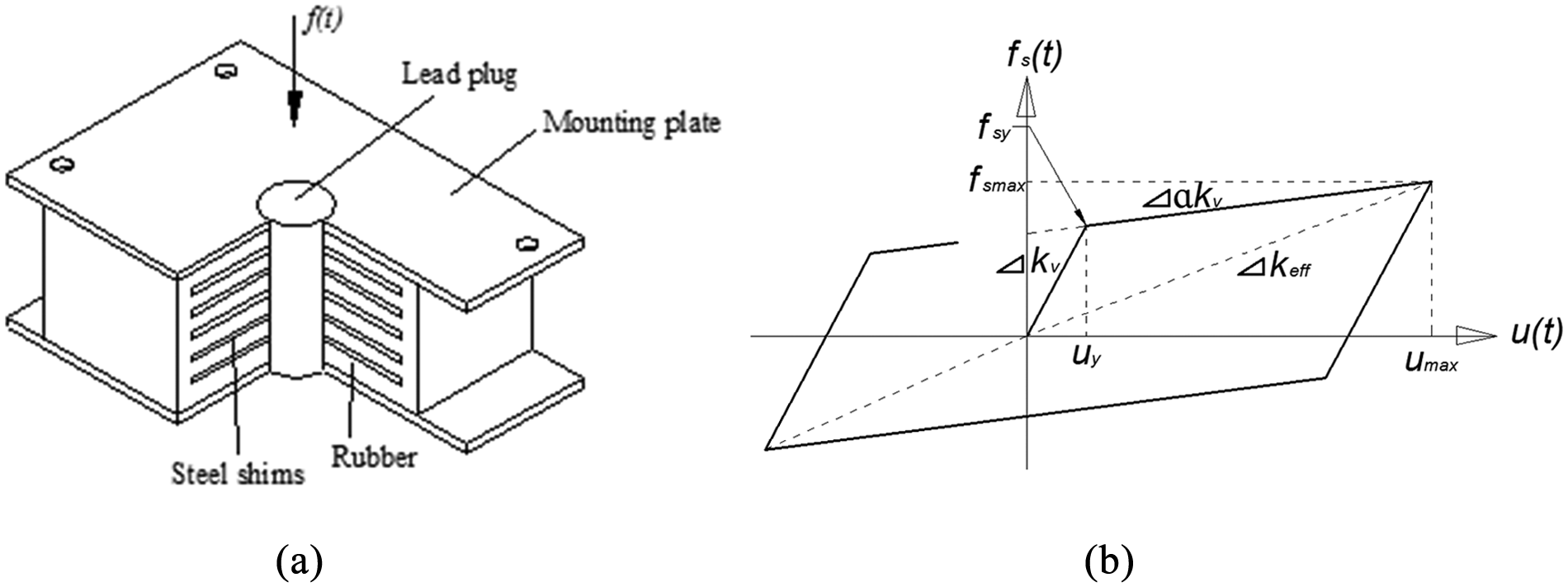
Typical lead elastomeric bearing used in bridges: (a) components and (b) force–displacement hysteresis loops.
Figure 1(b) represents a bilinear hysteretic model for simulating the response of a lead rubber bearing. In this figure,
Deterioration in elastomeric bearings is caused by external restraint forces which are generated in the movement of concrete in response to temperature, creep and shrinkage. The restraint may consist of friction at the bearings, bonding to already hardened concrete or by attachment to other components of the structure. Cracks resulting from the actions of external restraint forces develop in a similar manner to those caused by external load. Concern about the reliability of elastomeric bearings is increasing and studies on experimental and in-service bearings reveal the occurrence of permanent changes in the engineering properties of the bearings.4,5 Cyclic loading is found to cause progressive damage, analogous to fatigue in metals. 16 Most damage cases are in the form of progressive debonding between the rubber and steel shims. A degree of stiffness loss can be expected due to repeated cyclic loading causing breading of molecular bonds between polymers. 17 A method to characterize and monitor the structural parameters characterizing the bearing response is clearly needed.
Many methods have been proposed for parameter identification of single degree-of-freedom (SDOF) and multiple degree-of-freedom (MDOF) structural systems. Recently, wavelet ridges of continuous wavelet transform (CWT) have been employed to identify the instantaneous frequency (IF) of a time-varying structure, where the frequency change is gradual representing a linear system with time-varying frequency. 18 Nagarajaiah and Basu 19 investigate modal identification of linear time-variant systems and they conclude that the wavelet analysis is more appropriate than the Hilbert–Huang transform (HHT) in identifying changes in the frequency of linear systems due to the number of scales and coefficients that can be applied. Feldman 20 applies the Hilbert Transform (HT) to identify the non-linear instantaneous modal parameters of SDOF systems in forced and free vibration. However, the application of HT is limited as it only defines a ‘mono-component’ signal (i.e. obtain only one frequency value using a single component). 21 For ‘multi-component’ signals, the concept of IF becomes meaningless, given that the HT is inherently limited to ‘mono-component’ signals and breakdown of the signal components is needed. The signal needs to be defined in terms of its single ‘mono-components’ each having a different IF 8 as addressed by Huang et al. 22 They decompose the signal using Empirical Mode Decomposition (EMD) to obtain the Intrinsic Mode Functions (IMFs) and then use the HT to obtain the IF of the signal. This methodology is called the HHT and it is one of the most popular methods for analysis of non-linear and non-stationary data.22–24 In the following sections, the HHT is applied to the characterization of the response of non-linear systems with hysteresis that define lead rubber bearings. First, basics on the HHT are reviewed. Second, the mathematical model of the bearing (a SDOF) is introduced. Then, the response of the model to a time-varying force and to a sudden change in the force–displacement hysteresis loop is investigated via the HHT.
The HHT
There are two main steps in the HHT analysis process:22,25 EMD and the HT. The HT characterizes a time-domain signal
First step: EMD
The signal is decomposed into a number of IMFs using the ‘sifting’ process. The IMFs can be defined as a representation of oscillatory modes of variable frequency and amplitude that are time dependent, as opposed to simple harmonic functions of constant amplitude and frequency. The IMFs must satisfy two conditions:
The number of extrema and the number of zero crossings must differ by no more than 1.
The mean value of the envelope defined by the maxima and the minima at any given time must be 0.
The sifting process to obtain the IMFs is as follows:
Identify the local maxima and minima.
Find the mean m1(t) of the upper and lower envelopes.
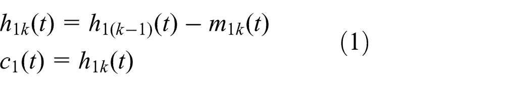
Obtain the difference
Check if
After the sifting process, (1)–(3) has been done a number of times, that is, k, the two conditions will be met and the first IMF,
However, too many sifting cycles could reduce all the components to a constant-amplitude signal with frequency modulation only, that is, only frequency variation is retained. To guarantee that the IMF components retain enough physical sense of amplitude and frequency modulations, the number of times, k, the sifting process repeats has to be limited. There are two main mathematical stoppage criteria proposed in the literature that are used to ensure that the sifting process stops when conditions (a) and (b) above are met:22,23
A first criterion based on limiting the normalized Square Difference (SD) between two successive sifting operations to a small value, that is

at time
A second criterion based on assuming the sifting process has ended after a predefined number of times. For instance, if after
The first criterion is difficult to implement in practice due to the need to select an accurate value of
The process of sifting starts by separating the finest local mode
Second step: the HT
Once the EMD process has been finalized, the second step of the HHT analysis is the HT of the IMFs.24,25 A complex analytical signal is formed for each IMF consisting of a real part defined as the

The complex signal can be expressed in exponential format as in equation (4)
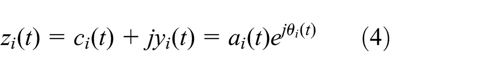
where

The IF

Using the HHT, it is possible to characterize the frequency of a non-linear system such as a non-linear support. The potential of the HHT in detecting changes in bearing stiffness is examined in the following sections.
Description of mathematical model of bearing
An elastomeric bearing is idealized as a SDOF system consisting of a mass (M) supported on a spring (

Bearing model: (a) SDOF and (b) force–displacement relationship.
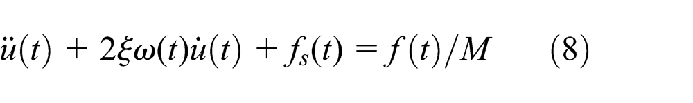
The response of the SDOF system in Figure 2 is governed by the dynamic equilibrium between the internal inertial (
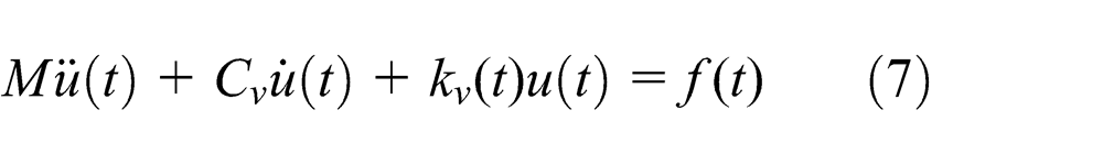
where
where

In equation (9),
The Bouc–Wen hysteretic displacement (


where
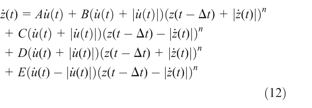
Equation (12) decouples the hysteretic loop in four loading regimes each of which being regulated by a different constant shape coefficient:
The main advantages of the model in equation (12) over the Bouc–Wen model in equation (11) is the added flexibility to the hysteretic cycle as each curve is defined separately. Setting the non-linear parameters B, C, D and E equal to 0 results in a linear relationship with a slope equal to that of the initial tangent slope. Depending on the selected coefficients, choosing a positive value shall bow the curve inwards (or outwards) from the loop, with the negative value producing the opposite effect.
Characterization of non-linear SDOF bearing model using the HHT
The response of the SDOF in Figure 2 (

In this theoretical test, the SDOF bearing model has a mass of M = 3135.8 kg and a viscous damping of 6% (ξ = 0.06).5,28,29 A vertical effective stiffness of 1.14375 × 10⁹ N/m is assumed which leads to an ‘effective’ natural frequency of 30.7 Hz. The following values are assigned to the constants of the hysteresis model of equation (12) to define the shape of Figure 2(b):
Figures 3(a) and (b) show the acceleration (

Response of the non-linear SDOF system to a sinusoidal load: (a) acceleration and (b) displacement.
The HHT is applied to the acceleration signal from Figure 3(a). Figure 4(a) and (b) show the first four IMFs resulting from the EMD process and the associated IFs via the HT, respectively. Although the total number of IMFs extracted from the acceleration is seven, only the first four IMFs are shown in the figure. The last three IMFs (IMF5–7) are residues of small magnitude that do not provide meaningful information on the system behaviour. Lower IMFs contain higher frequency components of the signal, and IMF1 appears to have higher coefficient values than other IMFs and to dominate the response.

HHT: (a) IMFs 1–4 using EMD; (b) associated instantaneous frequencies (IF1(t)–IF4(t)) in Hertz using the HT.
The frequency of the applied sinusoidal load (equation (13)) is 1.59 Hz and it is captured by IMF4 in Figure 4. The natural frequency of the SDOF system, NF(t), is time varying and determined in Hertz by

where the stiffness

Comparison of instantaneous frequency of IMF1 using HT and actual instantaneous natural frequency (NF(t)) of the system.
Figure 6 shows the variation of stiffness with time of the SDOF system using
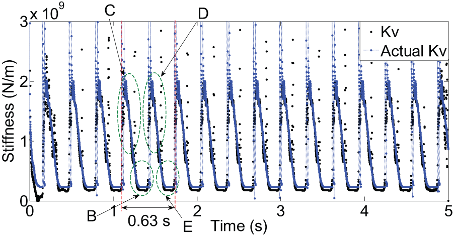
Comparison of stiffness prediction (
Although the IF1 and

PSD of acceleration in Figure 3(a).
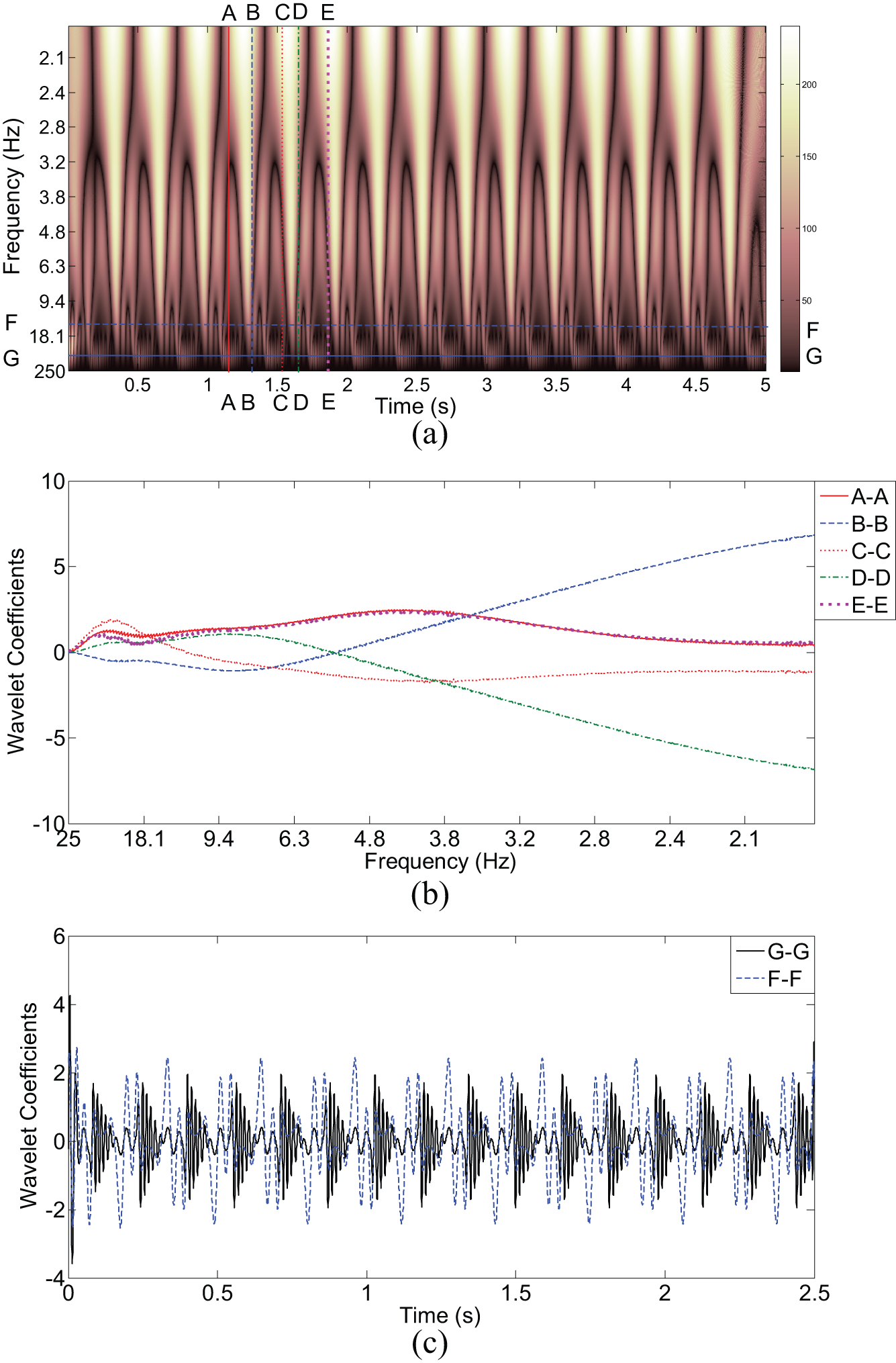
Wavelet analysis of acceleration in Figure 3(a): (a) contour plot of wavelet coefficients versus frequency and time, (b) wavelet coefficients versus frequency for times of 1.1, 1.225, 1.425, 1.54 and 1.73 s, and (c) wavelet coefficients versus time for frequencies of 41 and 14 Hz.
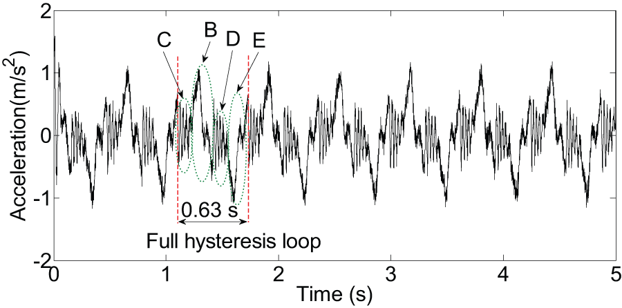
The CWT uses inner products to measure the similarity between a signal and a function known as the mother wavelet. In the CWT, the signal is compared to shifted and compressed or stretched (scaled) versions of the mother wavelet. By comparing the signal to the wavelet at various scales and points in time, a frequency–time map of wavelet coefficients is obtained. 33 Figure 8(a) shows the wavelet coefficients versus pseudo-frequency and time that result from applying the CWT to the acceleration response of Figure 3(a) using the Mexican Hat mother wavelet. The pseudo-frequency is directly proportional to the centre frequency of the wavelet in Hertz (for the Mexican Hat wavelet, this centre frequency is 0.25 Hz) and inversely proportional to the scale of the wavelet and to the sampling period. It is difficult to interpret the behaviour of the system from Figure 8 alone, so sections at times 1.1, 1.225, 1.425, 1.54 and 1.73 s (A-A, B-B, C-C, D-D and E-E, respectively) are plotted versus frequency in Figure 8(b) and sections at frequencies 14 and 41 Hz (F-F and G-G, respectively) are plotted versus time in Figure 8(c). In Figure 8(b), section A-A corresponds to the initial stage of C, while section B-B corresponds to the end of stage C and beginning of stage B. Sections through C-C and D-D correspond to the end of stage B and beginning of stage D. It can be seen that the sections C-C and D-D have the same magnitude than sections A-A and B-B, but they are in the negative region. Section E-E corresponds to the end of stage E and it is almost equal in magnitude to section A-A suggesting that the stiffness is returned to its original value and a full hysteresis cycle is complete. Figure 8(c) shows the variation in content of the pseudo-frequencies 14 and 41 Hz (lower and upper values respectively of the range of variation of the frequency of the system) with time. However, the range of variation of the frequency of the system, the frequency at which the system is responding for each point in time, and its duration are not as clearly defined by wavelets as in Figure 5 simply using the IF1(t) by HHT.
It has been shown that HHT can be used to characterize frequency and stiffness changes due to nonlinearity properties of a SDOF system, although one problem that may arise with the EMD process is over-decomposition of the signal resulting into excessive IMFs and mode mixing, that is, IMFs sharing similar frequencies. It is also important to note that this is a theoretical investigation of a SDOF system with a specific hysteretic loop and that experimental results may contain other complexities involving external factors such as temperature and/or inconsistencies of the applied load and the specimen and/or internal factors such as friction between steel shims and rubber (for steel-reinforced rubber bearings).
Identification of changes in the bearing behaviour using the HHT
Although the HHT was initially developed to characterize non-linear systems, its application to structural damage detection has been limited mostly to sudden losses in stiffness using simple periodic functions, experimental beams with crack or linear time-variant systems.19,34–37 The reason for this possibly lays on the lack of data to characterize how damage affects the overall performance of non-linear structural systems. In this investigation, damage is theoretically simulated through the introduction of a reduction in the effective stiffness of a hysteretic loop as shown in Figure 9(a). 38 The acceleration response of the SDOF system is illustrated in Figure 9(b) where a 10% reduction in effective stiffness is introduced after 2.5 s. This change in the effective stiffness of the hysteretic loop is visualized as an increase in the maximum amplitude of the acceleration signal of 0.282 m/s2 with respect to the original acceleration (i.e. maximum acceleration is 28.8% higher after the stiffness reduction). This large increase in acceleration is attributed to the low stiffness values experienced by the bearing at loading and unloading. In comparison, at higher stiffness, the change in acceleration is much lower (6.2%).

(a) Force–displacement relationship for the SDOF system before and after 10% loss in effective stiffness and (b) acceleration response before and after 10% loss in effective stiffness.
Four IMFs of interest can be obtained from Figure 9(b) using EMD, and the IFs of these IMFs are shown in Figure 10(a). Edge effects (before 0.5 s and after 4.5 s) appear in the IFs as a result of the decomposition process. 22 IF1(t)–IF4(t) show a sudden peak at the instant of change in effective stiffness. This peak can be clearly visualized in IF3(t) and IF4(t) of Figure 10(a), due to the relative high-frequency content at this location with respect to the rest of the IMF. The dominant IMF is IMF1 and Figure 10(b) zooms in on the IF1(t) shown in Figure 10(a). The average range of IF1(t) is 42.35–10.64 Hz prior to the simulated damage and 38.35–9.46 Hz after damage has occurred. Once edge effects are ignored, the reduction in frequency as a result of the stiffness change is 9.6% (−4 Hz) at the upper range (cases C and D in Figure 2(b)) and 11.1% (−1.18 Hz) at the lower range (cases B and E in Figure 2(b)). The average drop in stiffness is (9.6% + 11.1%)/2 = 10.35%, that is, approximately the 10% reduction in effective stiffness.

Instantaneous frequencies in Hertz before and after 10% effective stiffness loss of (a) IMFs 1–4 and (b) IMF1.
This section has demonstrated the capability of the HHT to extract important time–frequency information about the non-linear behaviour of a SDOF system. IF1(t) has been able to capture a small change in effective stiffness of 10%. It is acknowledged that experimental setups and more complex systems will require IFs from more than one IMF to gather sufficient information to characterize the system.
Influence of noise on the performance of the HHT
Noise can be caused by a number of factors which include the natural intermittent instabilities in the system, the concurrent phenomena in the environment where investigations are conducted, and/or the sensors and recording systems. As a result, data are always an amalgamation of signal and noise, that here they are simulated using the additive model

where
Acceleration response of the non-linear SDOF system to a sinusoidal load with 1% noise.
Following EMD of the corrupted acceleration signal, the corresponding IMFs 1–8 are represented in Figure 12(a) and (b). Compared to the noise-free signal (Figure 4), there is a higher number of IMFs that need to be considered as a result of the presence of noise. It can be seen that even low noise levels can have a significant impact on the decomposition process. Figure 12(c) and (d) shows the IFs associated with each IMF. IMFs 1–3 reveal high variability of frequency content between 0–500, 0–300 and 0–150 Hz for IMF1, IMF2 and IMF3, respectively, which can be attributed to noise. IMFs 4–8 contain a smoother variation of frequencies that appears to be in the range of IFs obtained in Figure 4(b) for noise-free acceleration.
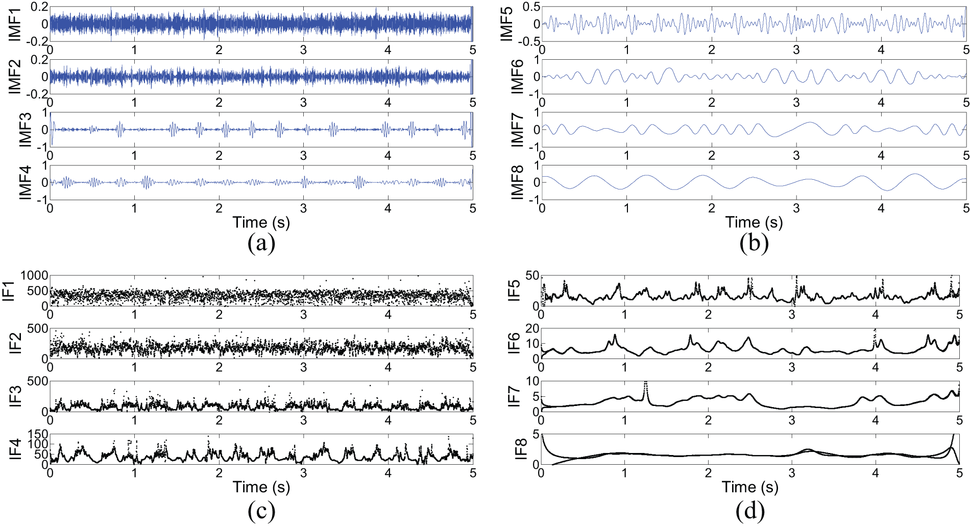
HHT for signal with 1% noise: (a) IMFs 1–4 using EMD. (b) IMFs 5–8 using EMD. (c) Associated instantaneous frequencies (IF1(t)–IF4(t)) in Hertz using the HT. (d) Associated instantaneous frequencies (IF5(t)–IF8(t)) in Hertz using the HT.
However, when plotting the IFs of IMF4 and IMF5 (Figure 12), together with the time-varying natural frequency of the system in Figure 13, the influence of noise is clear. The extraction of a clean IF that matches the frequency of the system is rendered unsatisfactory.
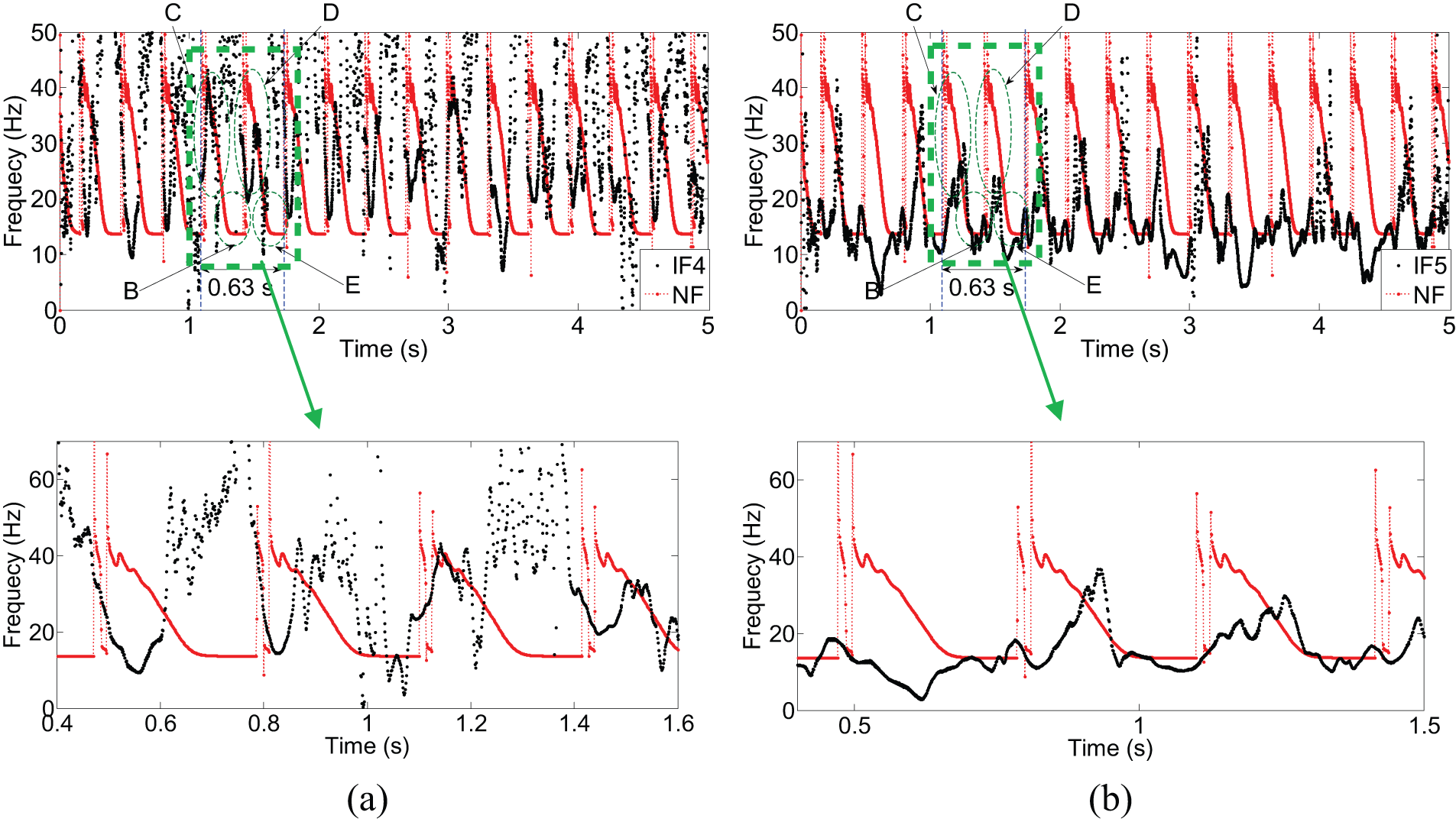
Comparison of the instantaneous frequency of IMF using HT on a 1% noisy signal and actual instantaneous natural frequency (NF(t)) of the system: (a) instantaneous frequency of IMF4 and NF(t) and (b) instantaneous frequency of IMF5 and NF(t).
For cases where noise has distinct time or frequency scales from those of the true signal, Fourier transform filters can be applied to separate the noise from the signal. Once the signal is filtered from noise, the HT has been shown to be capable of extracting phases and IFs for damage identification of linear scenarios.39,40 Similarly, sections ‘Characterization of non-linear SDOF bearing model using the HHT’ and ‘Identification of changes in the bearing behaviour using the HHT’ have demonstrated that the HHT is a valid tool to characterize instantaneous changes using the response of a non-linear SDOF bearing system where noise is non-existing or has been safely removed. However, traditional filtering methods may not be as reliable in separating mixed noise and harmonics in non-linear systems, and section ‘Influence of noise on the performance of the HHT’ has shown that the direct application of EMD and the HT to a corrupted signal can produce misleading results. In this regard, Ensemble Empirical Mode Decomposition (EEMD) 41 is an alternative to EMD that attenuates mode mixing and noise to some extent.
Conclusion
A hysteretic Bouc–Wen model has been implemented in a SDOF system to simulate the response of a lead rubber bearing. An IF analysis of the response of the SDOF via the HHT has provided information that allows characterizing the different stages of stiffness in this non-linear system (i.e. stages
Footnotes
Academic Editor: Andrea Spagnoli
Declaration of conflicting interests
The authors declare that there is no conflict of interest.
Funding
The authors would like to express their gratitude for the financial support received from the ‘PhD in Sustainable Development Programme’ at University College Dublin towards this investigation.