
Abstract
This article models the contact between the drillstring with large slenderness ratio and the extending rigid wellbore based on the multibody dynamics method. The drillstring is modeled as absolute nodal coordinate formulation beams with contact detection points. An algorithm is developed to locate the contact points and calculate the contact forces when the drillstring is sliding and rotating in the wellbore. This provides support force and friction for the moving drillstring and effectively confines it inside the wellbore. A rock penetration model is established based on the rock-breaking velocity equation. The governing equation for the full-hole drilling system including the drillstring and the contact model is established and solved. A rock penetration correction method is proposed to stabilize the computation and to model and simulate the slide drilling process. A field drilling process is modeled and simulated. The simulation result fits the experimental result well.
Introduction
In the past decades, there have been numerous theoretical and simulation investigations of the drilling process on predicting the wellbore and analyzing the drillstring’s motion and deformation.1–5 Conventional methods include the finite element method (FEM), the differential equation method, and other analytical solutions. Among them, analytical solutions are concise but have over-simplified the stochastic collision between the drillstring and the wellbore; FEM, although playing an important role in drilling process analysis, is not competent to modeling and simulating large deformation, large displacement, and rotation of the drillstring, and the large number of modeling elements greatly impairs the calculation speed.
The multibody dynamics approach has been adopted in drilling system analysis recently. This approach uses the absolute nodal coordinate formulation (ANCF) beam to model the flexible drillstring.6,7 This method enables modeling and simulation of the large deformation, large displacement, and rotation of the drillstring 8 with complex stochastic contact boundaries and slenderness ratio up to 103. The full-hole multibody dynamics drillstring model is thus developed and the simulation results greatly promote engineering understanding of the drilling process dynamics.
The drillstring–wellbore contact leads to friction and abrasion and may cause severe accidents like stuck-pipe incidents. A lot of studies have been carried out to analyze the contact.9–12 The bit–rock interaction model is another research focus. Theoretical and experimental work is performed to measure and model the contact force and the rock-breaking process.13–15 Some statics algorithms are also developed to directly predict the well trajectory in the stable drilling process.16,17
In this article, section “Modeling of the drillstring–wellbore contact and the bit–rock interaction” introduces a practical drillstring–wellbore contact model and a bit–rock interaction model. Section “Drilling system governing equation and solution” presents a multibody dynamics model of the drilling system, and the system governing equation is presented. When solving the governing equation, the rock penetration process is corrected at the end of each integration step. Simulation results are presented in section “Simulation result.”
Modeling of the drillstring–wellbore contact and the bit–rock interaction
Multibody dynamics model description of the drilling system
A schematic of the drilling system is shown in Figure 1.

Schematic of drilling system components.
The winch and the top drive control the translational and rotational motion of the drillstring. The drillstring bends and twists inside the wellbore. On the lower end of the drillstring, the bit pushes against the wellbore bottom and penetrates the layer.
In this article, the traveling block, the top drive and the bit are modeled as rigid bodies, and the drill line system is modeled as a spring with variable length and stiffness. The flexible drillstring is modeled with ANCF beam elements.
The drillstring rotates and slides downward in the wellbore and extends the wellbore with a cutting bit at the bottom to the designed direction. The 1000-m-long drillstring, hanging from ground, with a slenderness ratio above 103, surely would not work without contacting the wellbore. Torque from the top drive or a downhole motor nearby, combined with force from the drillstring, drives the bit to break the rock and thus to extend the wellbore. This makes the wellbore an extending tubular contact surface. Although the drillstring abrades the wellbore and the crustal stress slowly compresses the wellbore, the change in the wellbore section geometry is minor during drilling and is thus dismissed. At the lower end of the wellbore, the well bottom is a moving planar contact surface.
Contact detection points are fixed on the drillstring, so the detection points slide along the wellbore with the drillstring. In coiled tubing drilling, the contact points are evenly distributed on the drill pipe; in other drilling systems, there are tool joints along the drillstring. These tool joints are remarkably thicker than other sections of the drillstring and are the parts to plant detection points. Additional detection points are planted amid the tool joints when necessary. A special detection point against the well bottom is poised on the bit.
Modeling the wellbore
The wellbore is a rigid hole in the ground with a curved centerline and approximately circular cross sections. The wellbore’s centerline is called the well trajectory. A set of wellbore nodes are placed on the well trajectory. In petroleum industry, the well trajectory is described with the measured depth, the inclination, and the azimuth at each node, as shown in Figure 2. At a single point on the well trajectory, the measured depth refers to the arc length of the well trajectory from the starting point of the well, the inclination refers to the angle between the local tangent direction of the trajectory and the vertical downward direction, and the azimuth refers to the angle between the projection of the trajectory on the horizontal plane and the north direction.

Definition of well trajectory parameters.
Different methods have been developed to transform this set of three parameters to the form of the material coordinate (equals to the measured depth), the position vector, and the tangent direction vector of the well trajectory.18–20 To describe the wellbore geometry and the contact characteristics, the section radius and the sliding friction coefficient are introduced. Then, the wellbore between two nodes can be interpolated.
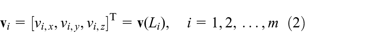
In this article, each wellbore node has nine parameters, which are the material coordinate, the position vector, the tangent direction vector of the well trajectory, the radius, and the coefficient of sliding friction of the wellbore, as shown in Figure 3. All these parameters are functions of the material coordinate.

Wellbore model.
Assume the wellbore has m nodes. The material coordinate at the ith wellbore node is

The radius of the wellbore at the ith wellbore node is

The coefficient of sliding friction of the wellbore at the ith wellbore node is

So, the wellbore is modeled using the material coordinate set


In this article, the cubic Hermite interpolation is applied to interpolating the well trajectory between wellbore nodes, as shown in Figure 4.

Wellbore interpolation.
The dimensionless local material coordinate between the ith and the i + 1th node is s, where

Thus, the parameters at each node are also the functions of s. The position vector


Assume the cross section of the wellbore is circular. The radius
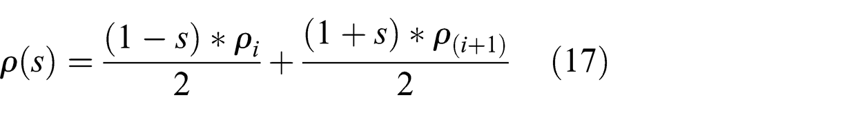
where
Assume the coefficient of sliding friction is continuous along the wellbore and is the linear interpolation of the coefficient of sliding friction at each node. The coefficient of sliding friction

where
Locating the contact point
The contact between the drillstring and the wellbore is to confine the drillstring inside the wellbore. Since the drillstring and the bit are always inside the wellbore, the penetration tolerance of the contact is unlimited. To locate the contact point P of a contact detection point D, we first locate the cross section passing P and then locate P on the cross section.
A bounding box method is used to find at which two nodes the contact point is between, as shown in Figure 5. C is on the well trajectory and marks the wellbore cross section.

Locating contact point.
In petroleum engineering, the curvature of the well trajectory is mostly less than 10°/30 m. The curvature radius of the well trajectory is much larger than the wellbore’s radius. Moreover, the wellbore’s radius is very uniform. Based on these facts, in the neighborhood of P, the wellbore and the drillstring are approximately cylindrical, so that the contact is cylindrical contact. This means D, C, and P are on the line of
Set an AABB bounding box for each node. Note
Then, we can get an extended AABB bounding box enclosing the ith and i + 1th bounding box. Successively check every extended bounding box, as shown in Figure 5. If point D is in the extended bounding box enclosing node i and node i + 1, it is very probable that point C is on the well trajectory between node i and node i + 1.
The precise position s of the contact point C can be located by Newton iteration. Note

Meanwhile, the derivative of this projection for the dimensionless local material coordinate s is non-zero, because

Obviously,

is convergent and has second-order convergence rate.
After iteration, if
Drillstring–wellbore contact force calculation
The contact force
where
The contact between two cylinders has been modeled with different methods. 21 Suppose the support force is a function of the penetration depth and the penetration velocity. Since the penetration tolerance is unlimited, the Hertz contact model is applied, and there is
where k is the contact stiffness coefficient, e is the contact recovery index, c is the contact damping coefficient,

Note

The magnitude of the friction is

where
The friction can be decomposed into the axial component and the circumferential component.
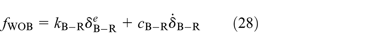
The axial component decelerates the axial motion of the drillstring. When pulling up, the friction increases the weight on hook (WOH) and may exceed the maximum WOH. When sliding down, the friction decreases the weight on bit (WOB; axial contact force on the bit from the well bottom) and thus decelerates drilling.
The circumferential component damps the rotation of the drillstring. In rotary drilling process, the circumferential friction increases the torque in the drillstring and may exceed the maximum torque of the drillstring and the top drive. In slide drilling process, when rotating the top drive a small angle to magnitude the bit attitude, the rotation in the drillstring is damped by the friction. The bit attitude control would be difficult. If the top drive rotates too quickly, the torque in the drillstring may accumulate and exceed the maximum torque of the drillstring and the top drive. In some other cases, the sudden release of the friction may lead to thread off, a severe accident in drilling.
Bit–wellbore contact force calculation
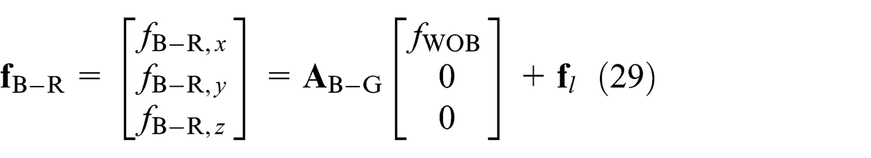
The well bottom is a moving contact surface, whose motion is defined in section “Instantaneous rock-breaking velocity calculation.” The track of the moving circular well bottom is the wellbore. Although the bit continuously cuts the well bottom and removes the rock, the bit still hits the static rocks at the well bottom, which is similar to the contact between a rigid ball and a plane. In this article, the bit is modeled as a rigid ball. The contact force
where
The lateral contact force
The transformation matrix from the bit body coordinate to the global coordinate is
The axial contact torque

where
Instantaneous rock-breaking velocity calculation
The well bottom moving velocity is commonly called the rock penetration velocity. In this article, to be distinguished from the contact penetration velocity, the well bottom moving velocity is called the rock-breaking velocity

where K is a coefficient describing the rock drillability,
Equation (31) is the three-dimensional (3D) drilling velocity equation for normal drilling process. This formulation is also valid for polycrystalline diamond compact (PDC) bits when the bit rotary speed is stable.
The magnitude of
The direct application of the instantaneous rock-breaking velocity may lead to calculation difficulties and very bad wellbore prediction quality. A two-stage correction method will be presented in section “Drilling system governing equation and solution.”
Drilling system governing equation and solution
System governing equation of the drilling system
The drilling system shown in Figure 1 is modeled as a rigid-flexible coupling system based on multibody dynamics method, as shown in Figure 6.

Bodies and constraints.
The crown block, the traveling block, the top drive stator, the top drive rotor, and the bit are modeled as rigid bodies. The crown block is fixed on the derrick. This constraint is modeled as a fixed joint to the ground.
The drill line between the crown block and the traveling block is modeled as a variable-length variable-stiffness extension spring. Suppose there are n pulleys in the traveling block. The length of the fast line (the drill line section connecting the winch) is
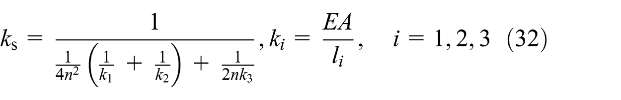
where E is Young’s modulus of the drill line, and A is the cross-sectional area of the drill line.
The motion of the winch leads to the length change of the drill line between the crown block and the traveling block, which is modeled as the length change of
The traveling block and the top drive stator are connected by a fixed joint. The top drive travels along a vertical rail on the derrick and is modeled as constrained by a translational joint with the ground. A revolute joint connects the top drive stator and the top drive rotor. The rotation between the top drive rotor and the stator is modeled as an angular velocity constraint.
To measure the output torque of the top drive, a very stiff torsional spring is added between the top drive rotor and the drillstring along the axis. The motion in the other five dimensions is constrained. The bit is fixed to the bottom of the drillstring.
There are five rigid bodies and six constraints in the drilling system. Based on the ANCF, the coordinate in this article is defined in the ground coordinate system.
The attitude of a rigid body or a beam node is described using the Euler rotation vector


The position coordinate of the ith rigid body is


where
An ANCF beam element is applied to modeling the drillstring. The cross section is assumed to be rigid, while shear is considered and the normal direction of the section is not along the centerline of the beam element. Suppose the beam element has n nodes, each with six generalized coordinates. The generalized coordinates of the nodes and the beam element are


where
The generalized coordinate at l in the beam element is interpolated as

where l is the arc length coordinate in the beam element and
Based on the rotation vector
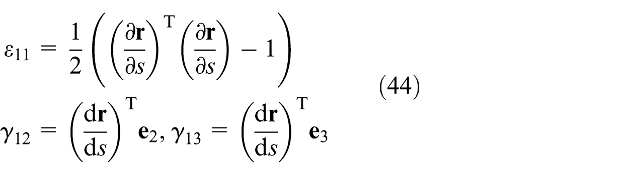
The curvature along the beam is

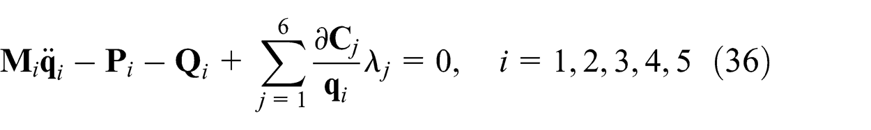
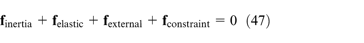
According to the d’Alembert’s principle, the total virtual work of the inertia force, the elastic force, the constraint force, and the external force (the contact force from the wellbore) are 0

The governing equation of the beam element is
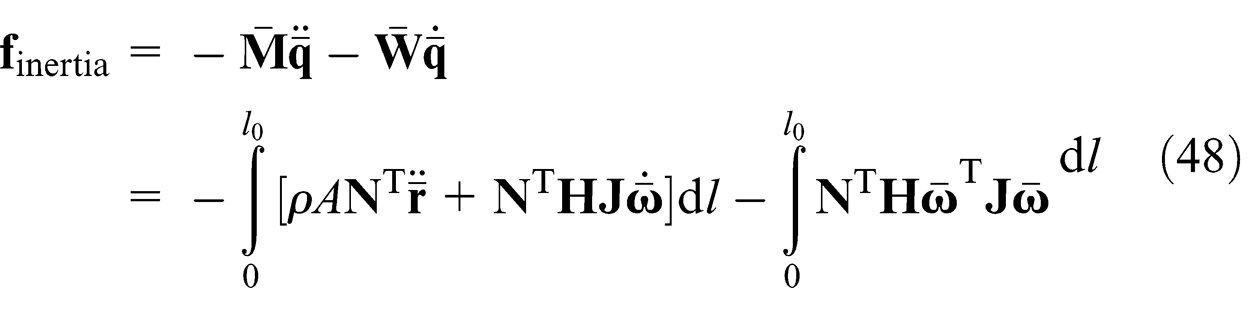


where

Note

Equation (47) becomes

According to equation (31), the rock penetration velocity
The time derivative of the position and the material coordinate of the well bottom node position are


The tangent direction vector of the bottom node is pointing to the direction of the rock-breaking velocity

Thus,

The radius
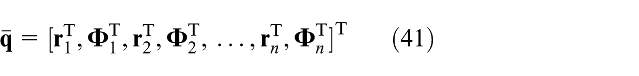
The system governing equation describing this highly coupled process is established using the Lagrange equations. The generalized coordinate is
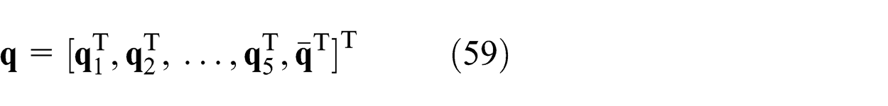
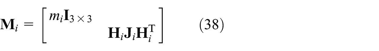
The generalized mass matrix is

The generalized forces are

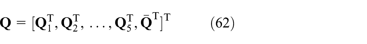
The governing equation of the drilling system is


Equation (63) is a differential algebraic equation (DAE). Equation (63a) is the dynamics equation of the bodies and is a combination of equations (36) and (54). Equation (63b) is the constraint equation for the rigid bodies and is from equation (37). Equation (63c) is the rock penetration equation and is a combination of equations (55)–(57). Thus, the rock penetration process is introduced into the system governing equation. The stiffness problem is converted into the DAE solving problem. A stiff DAE solver is essential to solving equation (63).
Solving the governing equation
Since the rock penetration process is very slow, the contact condition of the drillstring is almost unchanged before and after a single integration step. The solution sequence diagram is shown in Figure 7. At the kth integration step, the time is

Solution sequence diagram.
Suppose the initial wellbore has m nodes. A new wellbore node is added to the well bottom at the end of every integration step, and

The governing equation at the kth integration step is


The calculation process in each step is illustrated in Figure 8. In each integration step, the load condition and the motion state of the drillstring is first calculated in equations (65a) and (65b). Then, equation (65c) is calculated and the rock penetration result is acquired.
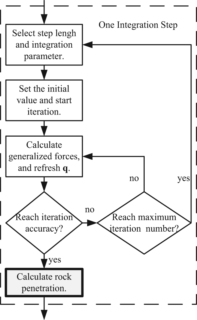
One integration step of solving the system governing equation.
In this article, the backward differentiation formula method is applied to solving the DAE. Based on this calculation strategy, the typical time consumption of the rock penetration calculation is about 0.1% of the total calculation time.
Rock penetration correction
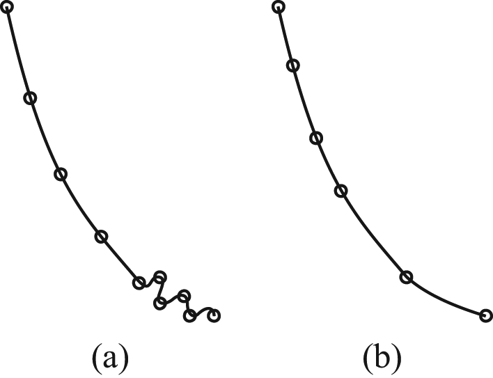
During the drilling process, the bit vibrates fiercely, and the direction of the instantaneous rock-breaking velocity calculated in a single integration step might be in any direction. The calculated wellbore will be highly curved, as shown in Figure 9(a), and should be corrected. A two-stage rock penetration correction strategy is applied at the end of each integration step, as shown in Figure 10.
Rock penetration process calculation with two-stage correction.

Stage II correction: (a) well trajectory before stage II correction and (b) well trajectory after stage II correction.
Stage I
At each integration step, the average rock-breaking velocity

with the bit direction as the new node tangent direction

Stage II
After every N integration steps, set the node tangent direction to be along the vector from the first node of the N nodes to the last node

Then, delete the first N − 1 nodes generated in the last N steps and reserve the Nth node, as shown in Figure 10.
The two-stage correction of the wellbore is essential for slide drilling system. The first stage stabilizes the calculation, and the second stage corrects the average rock-breaking velocity.
In stage I, the tangent direction of the new bottom node calculated in each step could only be the direction of the bit, as illustrated in Figure 11. If the direction of
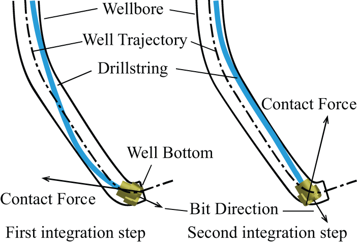
Initial contact between the bit and the wellbore bottom without stage I correction.
In stage II, the wellbore passes a low-pass filter, so that the zigzag in the well trajectory is diminished, as shown in Figure 9. A simulation result of the stage II correction is shown in section “Wellbore correction effectiveness.” In practical drilling process, there is a procedure after drilling called reaming, which makes the wellbore smoother and straighter. After reaming, the high-frequency oscillation in the well trajectory tangent direction is eliminated. So, the low-pass filter helps better approximate the real well trajectory. Moreover, in the compound drilling process (the process uses a slide drilling system but rotates the top drive to get a straight wellbore), none of the bit direction,
In addition, stage II correction reduces the wellbore nodes and thus reduces the storage cost and accelerates the contact point locating process.
Simulation result
Test oil well description
A full-hole multibody dynamics model of a slide drilling system in Bohai Sea, like the system shown in Figure 1, is established. The bottom hole assembly includes a PDC bit, a mud motor with a 1.25° bent housing, a float valve, a stabilizer, a measurement while drilling (MWD) system, and 14 heavyweight drill collars.
A rotary drilling process begins when the measured depth reaches 730 m and ends at the measured depth of 760 m. The initial inclination is 51° and the initial azimuth is 297°. The bit is initially off the bottom. At 250 s, the bit hits the well bottom and begins to break the rocks. The ROP is 32.7 m/h (9.08 mm/s). The WOH remains around 34 T. The angular velocity of the top drive is 53 r/min (5.55 rad/s). The torque of the top drive remains around
This compound drilling process is modeled and simulated, and the result is compared to the experimental result. The friction coefficient and the layer parameters of the wellbore are determined so as to make sure the simulated WOH and top drive torque are similar to the experimental results.
Wellbore correction effectiveness
In Figure 12, the helical red line is the original prediction of the well trajectory without stage II correction. Stage II correction makes the wellbore smoother and produces a new helix of much longer thread pitch, which is the blue line with pentagons.

The simulated well trajectory before and after stage II correction.
Well trajectory prediction quality examination
The MWD system records the inclination and azimuth while drilling and offers data to compare with the simulation result. Figures 13 and 14 show the horizontal and vertical projections of the well trajectory, respectively. The simulated well trajectory fits well with the experiment.

Horizontal projection of the well trajectory.

Vertical projection of the well trajectory.
Figures 15 and 16 show the inclination and the azimuth of the well trajectory, respectively. The wellbore in compound drilling process has a helical well trajectory. However, reaming enlarges the wellbore and turns the experiment wellbore from a thin helical hole to a thick straight hole. Additionally, the sampling rate of the MWD system is lower than the simulation result and reveals less information of the fluctuation of the well trajectory tangent direction. So, the experiment inclination and azimuth are nearly straight lines (the red lines with pentagons), while the simulation results are oscillating (the blue lines). The average inclination and the azimuth in simulation well fit the experiment data.

Inclination of the wellbore.

Azimuth of the wellbore.
Conclusion
In this article, the contact between the drillstring and the wellbore and the rock penetration process are modeled under the multibody dynamics method framework to model the drilling process. A rigid-flexible coupled multibody dynamics model of the drilling system is applied. The oil derrick components are modeled with rigid bodies, the drillstring is modeled with ANCF beams, and the bit is also considered a rigid body. Geometry and friction coefficient of the wellbore are interpolated from nodal values. Hertz contact forces between the contact points on the drillstring and the wellbore boundary provide support force and friction to the drillstring and effectively confine the drillstring inside the wellbore. A practical algorithm is developed to locate the contact points with respect to the Hermite nodes while the drillstring is carrying the contact points and sliding in the wellbore. On each step of the multibody system equation integration, the wellbore is extended at the bottom according to the 3D drilling velocity equation. A wellbore trajectory correction method is developed out of the detailed examination of the bit–bottom contacts within several integration steps.
A compound drilling process of 30 m in a 730-m-depth oil well in Bohai Sea is simulated. The average WOB, top torque, as well as the newly drilled well trajectory in the simulation results show very good correspondence with the collected field drilling data. The proposed method proves effective in drilling process simulation.
Footnotes
Academic Editor: Chuanzeng Zhang
Declaration of conflicting interests
The authors declare that there is no conflict of interest.
Funding
This work was supported by the Open Fund Project of the State Key Laboratory of Offshore Oil Exploration (Grant No. 2013-YXZHKY-020).