
Abstract
In order to simplify the design of path tracking controller and solve the problem relating to nonlinear dynamic model of autonomous underwater vehicle motion planning, feedback linearization method is first adopted to transform the nonlinear dynamic model into an equivalent pseudo-linear dynamic model in horizontal coordinates. Then considering wave disturbance effect, mixed-sensitivity method of H∞ robust control is applied to design state-feedback controller for this equivalent dynamic model. Finally, control law of pseudo-linear dynamic model is transformed into state (surge velocity and yaw angular rate) tracking control law of nonlinear dynamic model through inverse coordinate transformation. Simulation indicates that autonomous underwater vehicle path tracking is successfully implemented with this proposed method, and the influence of parameter variation in autonomous underwater vehicle dynamic model on its tracking performance is reduced by H∞ controller. All the results show that the method proposed in this article is effective and feasible.
Keywords
Introduction
As an important tool for marine development, autonomous underwater vehicle (AUV) has brought great benefits to human beings and it has great potential in both military and civil areas. AUV can complete the task of underwater detection, underwater cruise, and underwater communication in military areas. At the same time, AUV can be used for exploration and exploitation of marine resources, inspections of underwater facilities, and ocean rescue or salvage in civil areas. Autonomy and security are important characteristics of AUV. The meaning of autonomy is the ability to interact with the external environment and the most important aspect of autonomy is to have the ability of independent motion planning. 1 In addition, motion control technology is the foundation to realize long-distance navigation of AUV. The ability of motion control is an important technical support for AUV to complete various tasks. 2 Therefore, it has important theoretical significance and practical value to research the problem of AUV real-time motion planning and motion control.
As the key technology for AUV motion control, path tracking has attracted wide attention from scholars abroad in recent years and a large number of research findings are achieved in this area.3–7 Encarnacao and Pascoal 8 ensure robot trajectory to converge to the reference path globally and asymptotically through two-dimensional (2D) and three-dimensional (3D) nonlinear control strategy in Serret Frenet coordinate system. But uncertainties of model parameter and external disturbance factors such as ocean current are not considered in the design of controller. Silvestre C. adopts linear model in his research, designs a controller based on state feedback for different working points, and finally realizes the tracking control of piecewisely continuous terrain. But it is impossible to guarantee the global asymptotic stability of system 9 since nonlinearity and unmodeled dynamics in the model are not considered for this method. Borhaug and Pettersen 10 calculate tracking error of straight robot path in 3D space through line of sight (LOS) navigation algorithm. They apply cascade theory to design a stabilizing controller that guarantees K exponential stability of tracking error. In addition, Kaminer et al. 11 combine navigation method with control technology and finally realize straight path tracking of AUV through gain adjustment.
In this article, the problem relating to nonlinear dynamic model of AUV is considered while it is tracking a path in horizontal plane. Five sections are included in this article and organized as follows:
Feedback linearization method is adopted in section “Feedback linearization” and section “Linearization of AUV model” to make equivalent transformation of the nonlinear dynamic model.
Path tracking controller is easily realized in section “Design of H∞ controller” through simplification of AUV dynamic model. Parameter variation in AUV dynamics caused by marine environment is also studied in section “Design of H∞ controller” for improving the accuracy of tracking control. Mixed-sensitivity method of H∞ robust control is applied to design the tracking control law of state outputs (surge speed and yaw speed), and this method has been used widely in AUV motion control with well effect.
Section “Simulations” shows the simulation results of sinusoidal path tracking and circular path tracking. Corresponding analysis is also given in section “Sinusoidal path tracking” and section “Circular path tracking.”
Section “Conclusion” states conclusions of this article and the proposed method is also evaluated from view of application.
AUV feedback linearization
Feedback linearization
Feedback linearization is a method to transform nonlinear system into equivalent linear system through nonlinear feedback or dynamic compensation. Then, various control objectives can be achieved based on theory and methods of linear system. 12 In the research of feedback linearization, differential geometry method has been developed early and mainly includes state-feedback exact linearization13,14 and input–output decoupling linearization.15,16 Although great influence has been produced in nonlinear control field and a series of theoretical breakthroughs and achievements has been brought to the research on nonlinear control, there are still some difficulties in application of differential geometry method, which is relating to much more abstract mathematical theory. Another method in the research of feedback linearization is direct analysis method such as inverse system method17,18 developed in recent years. Theory of feedback linearization in nonlinear system keeps continuous improvement through research and introduction of some concepts and the results of the inverse system theory such as alpha-order integrating inverse system19,20 and pseudo-linear system.21,22
Linearization of AUV model
In this article, exact linearization with state feedback is applied to make coordinate transformation of nonlinear dynamic model based on the research of horizontal dynamics of AUV. Through equivalent transformation, a simplified pseudo-linear model is obtained from the complex nonlinear model of AUV and design of path tracking controller is largely simplified.
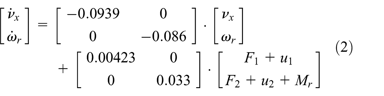
According to the dynamics model of “BEAVE” AUV proposed by Harbin Engineering University, 23 a nonlinear horizontal dynamics model used in this article is obtained and expressed as the following matrix form

where
If the following expression on motion relations is reasonable, namely

where Ds is the surge displacement and ψ is the yaw angle, state equations for AUV horizontal motion can be expressed as equation (4) through combining equation (2) with equation (3)
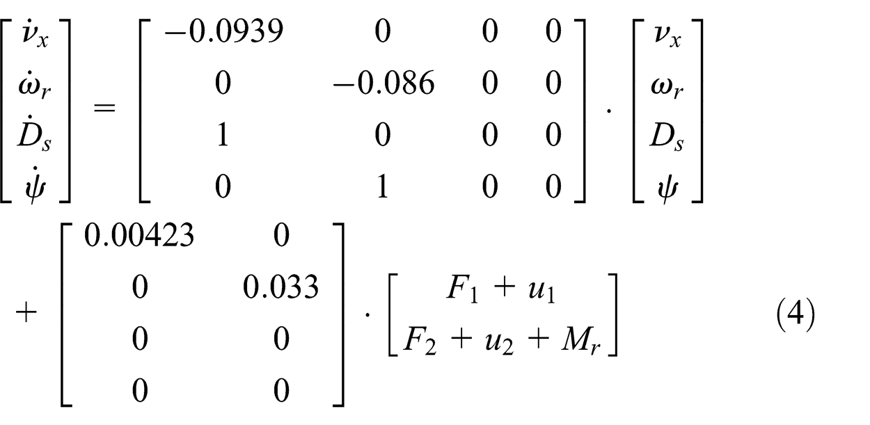
Equation (4) can be abbreviated as

where


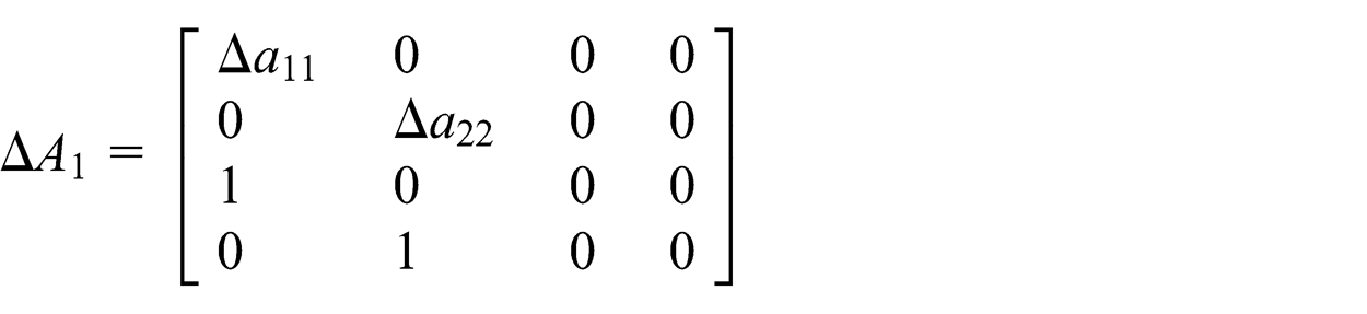
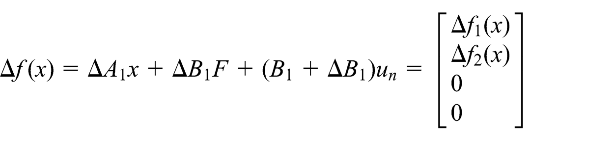
Considering uncertainty of hydrodynamic force coefficients and wave disturbance, it is possible to separate equation (5) into known nominal section and unknown uncertain section, namely

where

If the following variables are defined, namely


Equation (6) can be simplified and further transformed into equation (7)

Here, we cannot estimate the effects of Δf(x) and Δg on the horizontal motion attitude through precise calculation. Supposing disturbance satisfies matching condition, 24 namely


where


and uncertain terms in equation (7) are removed, state equations for nominal section can be obtained as shown in equation (8)

Relative degree of nominal system is calculated as follows


where gi is the column vector of g and hj is the component of h(x). According to equation (10), the total relative degree of system is 4, because relative degree corresponding to each output of system is 2. Thus, condition of realizing full decoupling and input-state linearization is satisfied. Each component of system output y = [Ds ψ] T is differentiated continuously and the following expression is obtained as shown in equation (11)
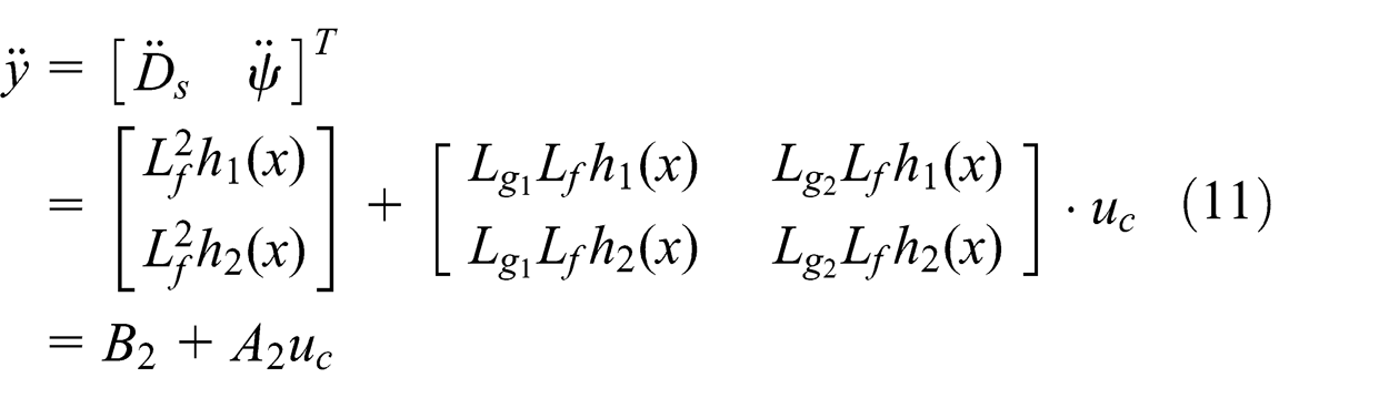
where

If control input of nominal system described by equation (8) is given, namely

where ue is the equivalent control input, second-order continuous differential of system output can be expressed as

From equation (14), it is obviously seen that surge acceleration and yaw angular acceleration can be controlled directly and then tracking of AUV position and its heading can be realized through designing the equivalent control input ue reasonably. Thus, process of controller design is largely simplified.
Control law for system input, namely, longitudinal propulsion force u 1 and rudder torque u 2, can be obtained through substitution of ue into equation (13).
Considering the effect of Δf(x) and Δg, coordinate transformation given by equation (15) is used according to the above matching condition of relevant disturbance terms
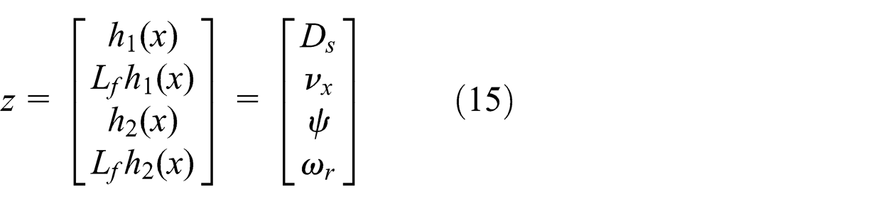
Through nonlinear coordinate transformation given by equation (15), system described by equation (7) can be linearized and decoupled into a pseudo-linear system, namely

where I 2 × 2 is a 2D identity matrix; A 3, B 3, and C 3 are the corresponding Brunovsky matrices, namely


Because equation (16) is equivalent to equation (7), robust controller can be designed for system model given by equation (16), first. Then, controller for system model described by equation (7) can be obtained through inverse coordinate transformation.
Design of H∞ controller
Considering characteristic of wave disturbance, H∞ controller design is based on mixed-sensitivity method according to control object model given by equation (16). S is the sensitivity function which is defined as the transfer function from reference input to tracking error. Sensitivity function embodies capacity of system restraining interference and parameter uncertainty. KS is the control sensitivity function which is defined as the transfer function from reference input to controller output. 25 If the characteristic of wave disturbance is known, amplitude of control input can be limited by setting control sensitivity function. According to the above definitions and model given by equation (16), S function and KS function are expressed in equations (17) and (18), respectively

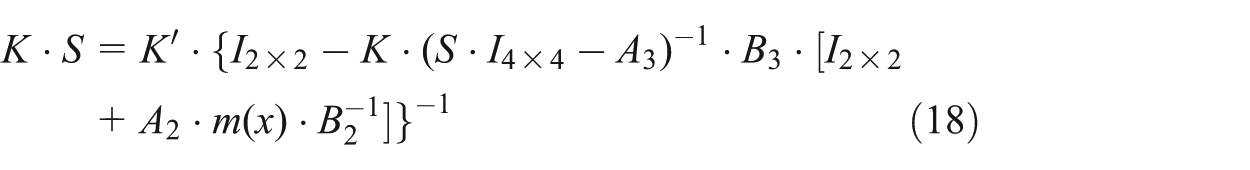
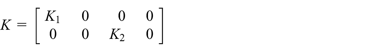
where K is the gain matrix of state feedback, namely


According to H∞ robust control theory,26–29 it is feasible to guarantee capacity of restraining wave disturbance and parameter uncertainty in tracking signal process by choosing proper weighted functions denoted by W 1(s) and W 2(s), which should satisfy the following inequality

namely


where La [] represents logarithm amplitude–frequency characteristic.
Choosing weighted function reasonably is key to design H∞ robust control system. W 1(s) is the weight of sensitivity function S and its amplitude decides system damping capacity on parameter uncertainty and disturbance. Considering frequency range of wave disturbance (0.1–3.0 rad/s), W 1(s) can be set as a low-pass filter with high gain in order to avoid parameter uncertainty, restrain disturbance, and track given signal accurately. W 2(s) is the weight of control sensitivity function KS and is used for limiting controller output in high frequency. While choosing W 2(s), it is important to make effect of wave disturbance attenuate at high-frequency band and limit controller output. To sum up the above factors, we set W 2(s) as high-pass filter. Thus, expressions of W 1(s) and W 2(s) are given as follows

In gain matrix of state feedback, unknown parameters (e.g. K 1, K 2) can be determined by placing corresponding poles of closed-loop system according to the expectation values of performance index. Then mixed-sensitivity function can be calculated through equations (17) and (18). Finally, the two inequalities about logarithm amplitude–frequency, namely, inequalities (20) and (21), should be tested. If inequalities (20) and (21) are not satisfied at the same time, K 1 and K 2 need to be reset. After K 1 and K 2 are determined, equivalent control input of pseudo-linear system model is substituted into equation (13), and control law of original system before linearizing can be obtained and expressed by equation (22)

Bode figure of mixed-sensitivity transfer function is shown in Figure 1, from which it is obviously seen that logarithm amplitude–frequency always keeps lower than 0 dB, namely, inequality (19) is satisfied. Bode figure of sensitivity function S and 1/W 1 is shown in Figure 2, where logarithm amplitude of sensitivity function attenuates in the frequency range lower than 0.1 rad/s, and disturbance with low frequency is obviously restrained. Within the whole frequency range, logarithm amplitude of S always keeps lower than that of 1/W 1. So, condition of inequality (20) is satisfied. Bode figure of control sensitivity function KS and 1/W 2 is shown in Figure 3, where controller output is effectively limited in high-frequency range, namely, amplitude and frequency of rudder angle are both limited. Thus, requirement of inequality (21) is also satisfied through proper selection of weighted function W 2. Figures 4 and 5 show the amplitude–frequency characteristics and the phase-frequency characteristics of nominal plant, respectively. Nichols curves of nominal plant are given in Figure 6.

Bode figure of mixed-sensitivity function.
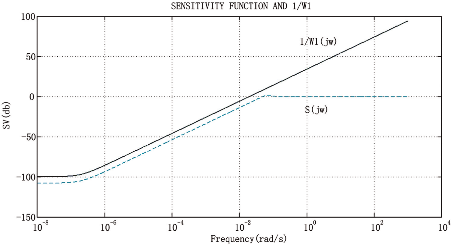
Bode figure of sensitivity function S and 1/W 1.

Bode figure of control sensitivity function KS and 1/W 2.

Amplitude–frequency characteristics of nominal plant.

Phase-frequency characteristics of nominal plant.

Nichols curves of nominal plant.
Simulations
Sinusoidal path tracking
In order to verify the control performance of AUV path tracking, simulations are conducted to prove effectiveness of H∞ controller while AUV follows a given sinusoidal path with varying dynamic model parameters. The desired sinusoidal path is expressed as
Initial condition of AUV path tracking is given by

Uncertain parameters in AUV dynamic model are described as

where a 1, a 2, b 1, and b 2 are the corresponding normalized values of hydrodynamic force coefficients, and Δa 1, Δa 2, Δb 1, and Δb 2 represent their corresponding uncertain sections. Figure 7 shows the simulation curve of AUV following given sinusoidal path. Figure 8 shows sinusoidal path tracking errors in horizontal plane. The tracking error in X-direction is holding at −0.0104 m, and the tracking error in Y-direction keeps within the range [0.0058 m, 0.0064 m]. Figure 9 shows simulation curves of control input for sinusoidal path tracking. Propulsion force finally varies between −0.0114 and 0.0114 N. Rudder torque fluctuates near 0 with the maximum amplitude 0.002 N m. Figure 10 shows curves of AUV states in sinusoidal path tracking. Surge speed varies between 1.0002 and 1.1808 m/s finally. Yaw angular rate and yaw angle fluctuate within the range [−2.2609°/s, 2.2609°/s] and [−32.1249°, 32.1249°], respectively.

Simulation of AUV following given sinusoidal path (H∞ robust control).

Curves of sinusoidal path tracking errors (H∞ robust control).
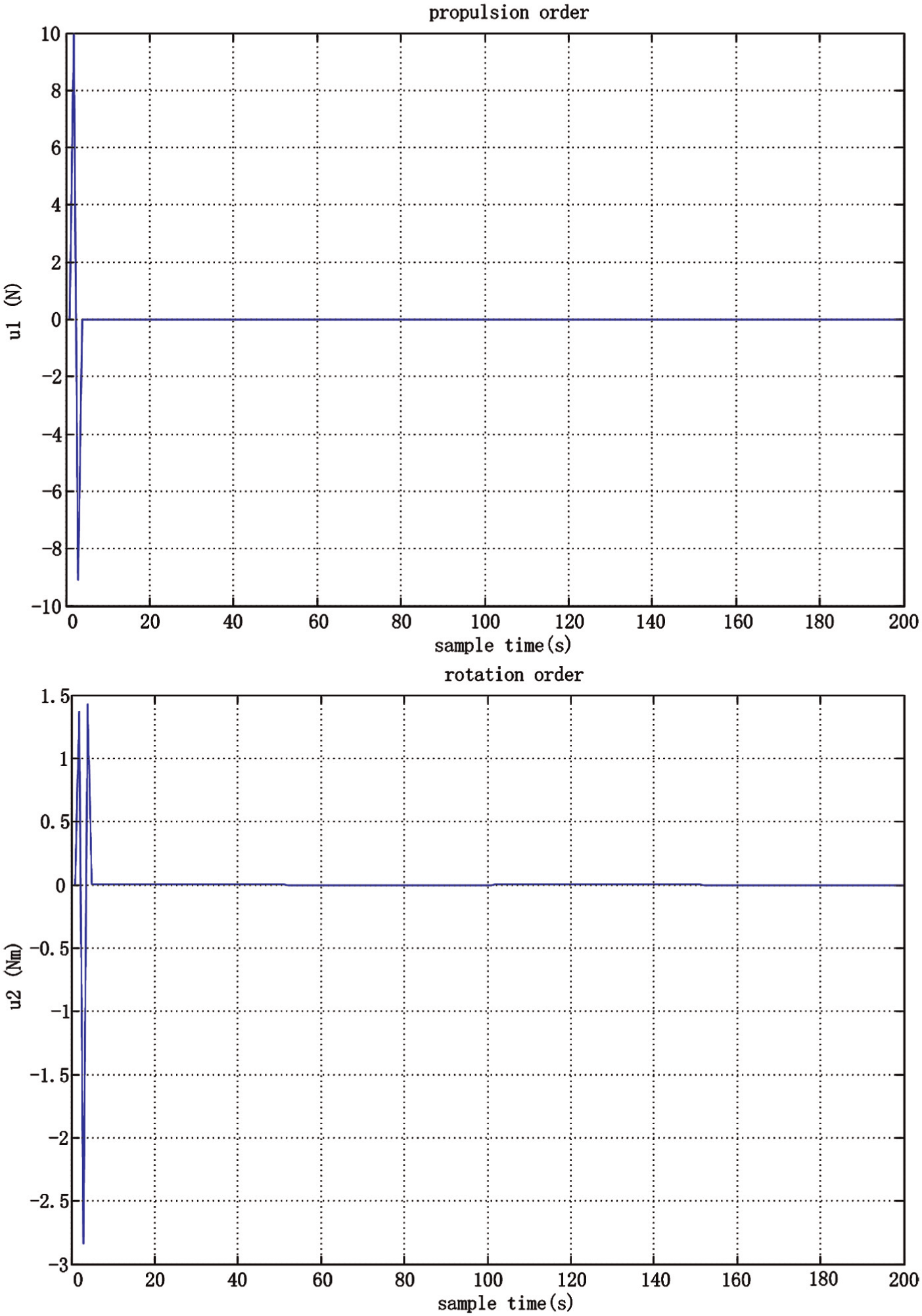
Curves of AUV control input (following sinusoidal path through H∞ robust control).

Curves of AUV states (following sinusoidal path through H∞ robust control).
Figures 11 and 12 show the performance of proportional–integral–derivative (PID) control for sinusoidal path tracking. Three key parameters of PID control are set as P = 0.72, I = 0.38, and D = 0.11, which are designed based on the nominal part of AUV dynamic model, namely


Simulation of AUV following given sinusoidal path (PID control).

Curves of sinusoidal path tracking errors (PID control).
When a 1, a 2, b 1, and b 2 vary with different sea conditions, the above parameters of PID control are not appropriate for sinusoidal path tracking as shown in Figures 11 and 12. Tracking errors in X-direction and Y-direction both increase with time, and the error maximum in X-direction even reaches 3 m, which is unsatisfied for designers in any case. From this point of view, performance of PID control for sinusoidal path tracking is rather worse than H∞ control method proposed in this article. Robustness of H∞ control is quite better than PID control, and the former is more suitable for AUV path tracking. PID control is only applicable to a certain stable condition and requires a combination of adaptive strategy to improve its robustness.
Circular path tracking
Simulations of circular path tracking are conducted for further verification. Figure 13 shows the effectiveness of H∞ controller while AUV follows a given circular path with varying dynamic model parameters. Circular path is expressed as

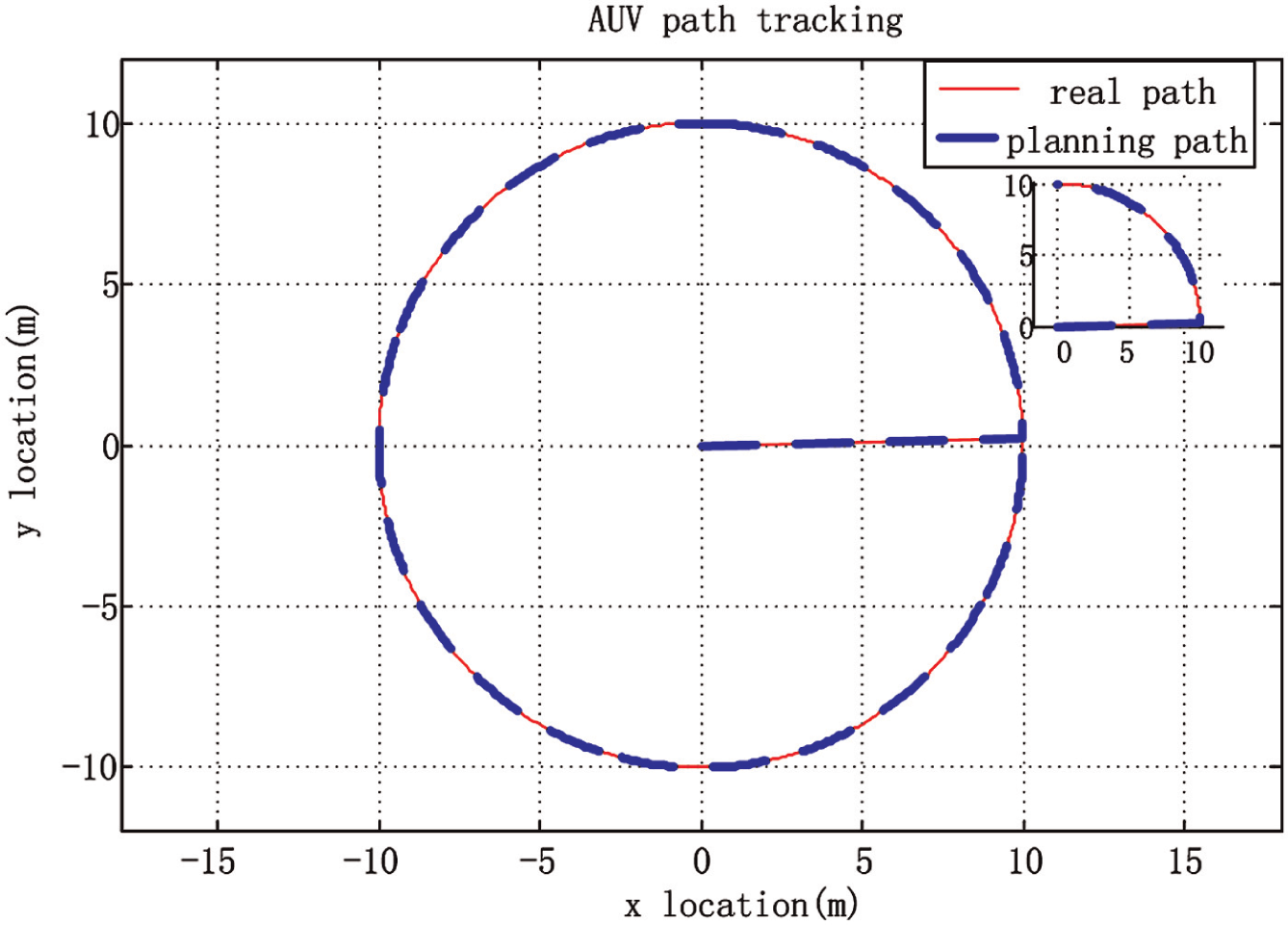
Simulation of AUV following given circular path (H∞ robust control).
Initial condition of AUV path tracking is given by

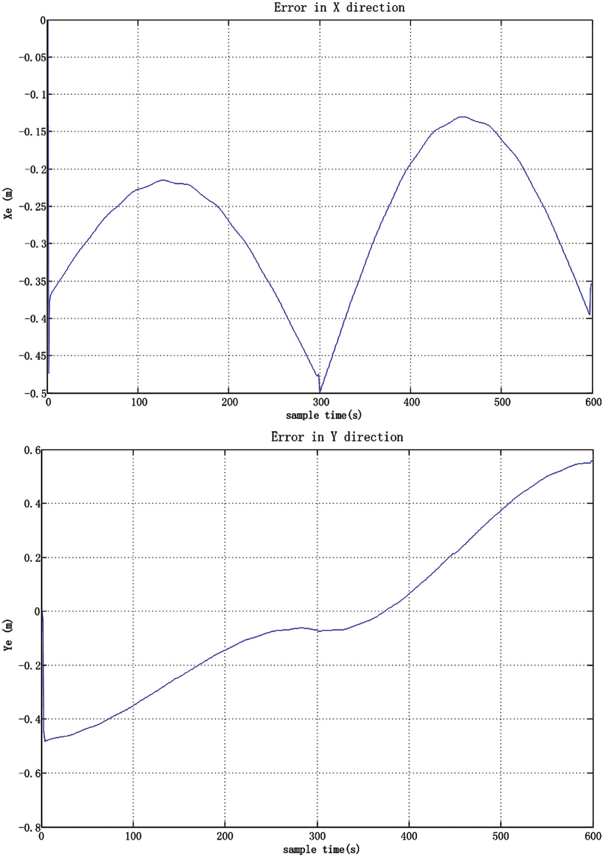
Uncertain parameters in AUV dynamic model vary with the same regularity described in section “Sinusoidal path tracking.”Figure 14 shows circular path tracking errors in horizontal plane. The mean values of tracking error in X-direction and Y-direction are 0.0051 and −0.0048 m, respectively. Figure 15 shows simulation curves of control input for circular path tracking. Propulsion force is finally holding at 0. In path tracking process, the maximum of rudder torque is 0.3927 N m which is smaller than the corresponding threshold of rudder design. Figure 16 shows curves of AUV states in circular path tracking. Surge speed remains 0.013 m/s finally. The maximum of yaw angular rate is −22.4141°/s which meets the constraints of AUV state, and yaw angle varies from 90° to −90° periodically.

Curves of circular path tracking errors (H∞ robust control).

Curves of AUV control input (following circular path through H∞ robust control).

Curves of AUV states (following circular path through H∞ robust control).
Figures 17 and 18 show the performance of PID control for circular path tracking. The PID control parameters are set as P = 0.81, I = 0.43, and D = 0.15, respectively, which are designed based on the nominal part of AUV dynamic model. When the coefficients in this dynamic model vary frequently, the above parameters of PID control are not appropriate for time-varying model of AUV motion. As shown in Figure 18, the error maximum in Y-direction even reaches 0.6 m. From Figures 13 and 17, it is obviously seen that performance of PID control for circular path tracking is rather worse than H∞ control when the parameters of AUV dynamic model are time-varying. Robustness of H∞ control is fairly well and more suitable for varying sea conditions in comparison with PID control.

Simulation of AUV following given circular path (PID control).
Curves of circular path tracking errors (PID control).
As shown in Figures 7, 8, 13, and 14, performance of H∞ controller designed in this article is favorable when AUV follows a given path with varying dynamic model parameters. The path realized by H∞ controller is consistent with the given path. Favorable robustness of closed-loop system demonstrates that the designed controller is effective on restraining parameter variation in AUV dynamic model.
As shown in Figures 9, 10, 15, and 16, state output and control input of dynamic model both satisfy the constraints of AUV maneuver when H∞ controller is used for AUV path tracking. Thus, implementation of the scheme is feasible, based on which planning path tracking is realized. H∞ controller guarantees tracking control performance is not influenced by variation in AUV dynamic model. So, there is certain theoretical significance and application value for H∞ control used for solving path tracking problem.
Conclusion
Considering nonlinearity and parameter uncertainty of AUV dynamic model in horizontal plane, H∞ controller for AUV path tracking is designed by using feedback linearization method and H∞ robust control theory in this article. This H∞ controller can make the performance of path tracking not influenced by model disturbance when the coefficients in AUV dynamic model vary with the effects of marine environment. Favorable simulation results of tracking a given path demonstrate that the new method proposed in this article is considerably effective and feasible for solving the problem of parameter variation in AUV dynamic model, which often occurs during the process of path tracking.
Footnotes
Academic Editor: Xiaotun Qiu
Declaration of conflicting interests
The authors declare that there is no conflict of interest.
Funding
Portions of this work were performed under the projects supported by National Natural Science Foundation of China (Grant No. E091002/50979017), PhD Programs Foundation of Ministry of Education of China and Basic Technology (Grant No. 20092304110008), Research Operation Item Foundation of Central University (Grant No. HEUCFZ 1026), and Harbin Science and Technology Innovation Talents of Special Fund Project (Outstanding Subject Leaders) (Grant No. 2012RFXXG083).