Torsional stress in non-circular cross sections by the finite element method

Abstract

The presented work is used to develop a new numerical calculation program to determine the torsional stress in simply connected non-circular cross sections of a beam subjected to a constant torque using the finite element method. The method used is the finite element quadrilateral element with four nodes. The boundary conditions are of Dirichlet. In applications for torsion usually formulas and results for the circular section are used, although the section in the case of type real and not circular. This is due to lack of form for non-circular sections in general. Each section has its own form of the twist angle and strain which is different from one section to another. This formula is connected with the polar moment of inertia if the section is circular and different if the section is not circular. Hence, our interest is directed toward calculating polar moment of inertia and constant torque if the section is not circular. The results presented are chosen for simple sections for comparison and other complex shapes such as airfoil having a physical and practical interest. A calculation error between the theoretical results and the calculated results is done in this context.

Introduction

In the past, researchers used the experimental method to demonstrate and validate their theories and assumptions of scientific research that does not have an analytical estimate. But when natural phenomena are too complex, dangerous, expensive, or long to reproduce in an experiment, it was necessary to create a simplified process, currently named the numerical simulation. ¹

This study will then perform a numerical calculation to determine the stress distribution of cylindrical torsion beams of arbitrary non-circular section. Indeed, the complexity of this section induces that the exact solution does not exist, and of course our interest is directed toward the search for approximate numerical solutions. The finite element method was introduced and applied successfully since it adapts well to any selected section. ¹

The resistance of the materials gives theoretical relationships only for torsion of the cylindrical circular sections. But for an aircraft, most of the structures are non-circular. We talk about the wing, fuselage, drift, spars, blades, blade of a helicopter, and others involving the field of mechanical engineering. ¹

Traction and compression loading, bending, and torsion are the three fundamental modes of loading which can act on right prismatic beam. In this work, we study and focus on the issue of torsion. We find this latter mode of loading, alone or in combination with others, in a large number of structural elements and machine. ²

To study the torsion of a beam of non-circular section, we use the more general methods derived from the elasticity theory.^1–4

Figure 1 illustrates the deformations undergone by a beam of circular cross section and the other square section subjected to a torsional moment. In general, a planar section normal to the longitudinal axis of the frame may still be plane after deformation.

Figure 1.

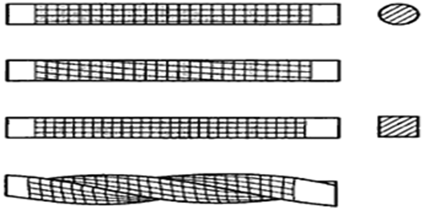
Deformation due to a torsional moment in a beam of circular cross section and the other non-circular.

Equations of discretization managing the phenomenon of torsion are based on the finite element method (two-dimensional (2D)) whose main advantage is to provide a good representation of complex geometries, but relatively heavy enough volume and computation time.^1,4–6

However, two main difficulties meet if the finite element method is used. The major difficulty is the optimal mesh generation and adaptation of the mathematical model equations. Another difficulty is the choice of appropriate numerical method to solve the algebraic system of equations given the large number of degrees of freedom.^4,7–10

To do this, we must divide the field into small sub-domains of simple geometry known as the quadrilateral geometry through interpolation functions. A large number of finite elements are developed and implemented for the development of a numerical program to have a suitable convergence.^4,5,8

Given the large size of the stiffness matrix, stored in the computer memory will be carried out using the technical of matrix bands to avoid storage boxes zero. To have a large number of zeros must be make a good numbering of mesh nodes.^11–16

Similarly, solving the system of equations will be done by using the direct algorithm of Khaletski and will be modified specifically for bands and symmetric matrices.^4,14–16

The solution of the problem is presented by the distribution of the flux of stress in the field which can be easily transformed to the distribution of torsional stress. A calculation of the integral of the flux stress distribution is of great interest to determine the formula for the unit angle of twist applied only to the selected section. ⁴

A very important parameter is represented by calculating polar moment of inertia of the selected section. The polar moment of inertia I is enters in the formula of the torsion angle unit. Note that this constant is equal to the torsion polar moment of inertia for the circular section and is different for other sections. ⁴

Analysis of the Prandtl equation by the finite element method

The finite element analysis is complicated by the fact that problems in two dimensions are described by partial differential equations. The contour Γ of the domain Ω in two dimensions is in general a curve.^3,5

However, the finite elements have simple geometric shapes that can be used as an approximation to the data field in two dimensions. On the other hand, for 2D problems, we do not seek only an approximation of the solution for partial differential equations’ data but also an approximation of the field given by a suitable mesh finite element. ⁵

Therefore, we will obtain a good approximation of the error (due to the approximation of the solution) as the discretization error (due to the approximation of the domain) in the analysis of problems of finite elements in two dimensions.^5,8,17

The finite element meshes for the simple elements such as 2D quadrilaterals are connected together by nodes on the contour of the element.^4,9,18,19

The opportunity to represent the geometry of the collection area by finite element method makes it a valid and a practical tool for solving boundary value problems.^5,6,8,17,20 This is a differential equation of second-order, linear, and elliptic type associated with the boundary conditions of the first order of Dirichlet said in an arbitrary planar domain Ω (x, y) ⁴

$$\frac{{\partial }^2\Phi }{\partial x^2}+\frac{{\partial }^2\Phi }{\partial y^2}=-2G\theta ;\Phi =0\mathrm{on}\Gamma$$

(1)

$${\tau }_{\mathrm{xz}}=\frac{\partial \Phi }{\partial x},{\tau }_{\mathrm{yz}}=-\frac{\partial \Phi }{\partial y}$$

(2)

$$M_t=2\int \Phi (x,y)\mathrm{dxdy}$$

(3)

The plan reported on the section is the (xGy). To solve a problem of torsion, it suffices to calculate the values of the four unknowns Φ, τ_xy , τ_xz , and θ, using equations (1)–(3). Subsequently, Prandtl introduced the concept that we can solve the problem of torsion by calculating the value of a single unknown, called stress function Φ (x, y). This function is differentiable and is associated with the constraints according to relation (2). ⁴

If it is assumed that Φ = 2Gθu in equation (1), we have the following form^4,5

$$\frac{{\partial }^{2}u}{\partial x^2}+\frac{{\partial }^{2}u}{\partial y^2}=a;u=0\mathrm{on}\Gamma$$

(4)

with a = −1.

And

$$\frac{{\tau }_{\mathrm{xz}}}{G\theta }=2\frac{\partial u}{\partial x},\frac{{\tau }_{\mathrm{yz}}}{G\theta }=-2\frac{\partial u}{\partial y}$$

(5)

$$\theta =\frac{M_t}{\mathrm{GC}}$$

(6)

with

$$C=4\int u(x,y)\mathrm{dxdy}$$

(7)

We develop the variational form of equation (4) for a typical element by multiplying the equation by a test function ν(x, y), which once assuming differentiable with respect to x and y, and then integrated into the area of the element (Ω^e), we have^4,5

$$0=\underset{{\Omega }_e}{\int }[\frac{\partial \nu }{\partial x}\frac{\partial u}{\partial x}+\frac{\partial \nu }{\partial y}\frac{\partial u}{\partial y}-\nu a]\mathrm{dxdy}$$

(8)

Equation (8) is the basis of the variational form of the finite element model of equation (4).

Finite element formulation

The variational form of equation (4) indicates that the approximation of u must be chosen at least bilinear in x and y. Suppose u is approximated by the following expression^4–8

$$u(x,y)={\displaystyle \sum _{j=1}^{j=n}}{u}_j{N}_j(x,y)$$

(9)

Specifies the form of N_j (x, y) will be developed for the four-node quadrilateral element (see Figure 2). Substituting equation (9) in variational form (8), we obtain

$${\displaystyle \sum _{j=1}^{j=n}}{K}_{\mathrm{ij}}^{(e)}{u}_j^{(e)}=F_i^{(e)}$$

(10)

Figure 2.

Quadrilateral element has four nodes decomposed into two triangles.

as

$$K_{\mathrm{ij}}^{(e)}=\underset{{\Omega }_e}{\int }[\frac{\partial N_i}{\partial x}\frac{\partial N_j}{\partial x}+\frac{\partial N_i}{\partial y}\frac{\partial N_j}{\partial y}]\mathrm{dxdy}$$

(11)

and

$$F_i^{(e)}=\underset{{\Omega }_e}{\int }{\mathrm{aN}}_i\mathrm{dxdy},i=1,2,\dots ,n$$

(12)

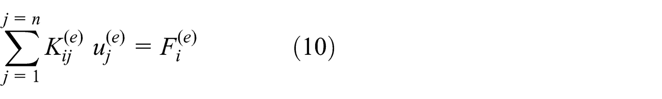
Equation (10) represents the mathematical model of the finite element for equation (4).^4,5

An examination of variational form (8) and stiffness matrix of the finite element equations in equation (11) shows that the function N(x, y) must be at least a bilinear function in x and y. So, there is a correspondence between the number of nodes in the element and the number of terms in the polynomial approximation of a dependent variable.

For 2D problems, the correspondence between the number of nodes (which is equal to the number of terms of polynomial approximations) and the degree of polynomial is not unique. In our case, the polynomial

$$u(x,y)=c_1+c_{2}x+c_{3}y+c_4\mathrm{xy}$$

(13)

contains four terms (linearly independent), linear in x and y. This approximation requires an element with four nodes, where one chooses a quadrilateral with nodes at vertices as shown in Figure 2. One can use approximation (14) instead of following approximation (13). It also contains four constants generalized and is symmetrical. But in our study, we are interested in relation (14)^{4–6,8,17,20}

$$u(x,y)=c_1+c_{2}x+c_{3}y+c_4(x^2+y^2)$$

(14)

Functions of interpolations

We must rewrite approximation (13) so that it satisfies the conditions of the nodes’ vertices of a quadrilateral by

$$\{\begin{array}{c}\hfill u_1=u(x_1,y_1)=c_1+c_2{x}_1+c_3{y}_1+c_4{x}_1{y}_1\hfill \\ \multicolumn{1}{c}{u_2=u(x_2,y_2)=c_1+c_2{x}_2+c_3{y}_2+c_4{x}_2{y}_2}\\ \multicolumn{1}{c}{u_3=u(x_3,y_3)=c_1+c_2{x}_3+c_3{y}_3+c_4{x}_3{y}_3}\\ \multicolumn{1}{c}{u_4=u(x_4,y_4)=c_1+c_2{x}_4+c_3{y}_4+c_4{x}_4{y}_4}\end{array}$$

(15)

we put

$$\{u\}=\left\{\begin{array}{c}\hfill u_1\hfill \\ \multicolumn{1}{c}{u_2}\\ \multicolumn{1}{c}{u_3}\\ \multicolumn{1}{c}{u_4}\end{array}\right\},[H]=\left[\begin{array}{cccc}\hfill 1\hfill & \hfill x_1\hfill & \hfill y_1\hfill & \hfill x_1{y}_1\hfill \\ \multicolumn{1}{c}{1}& \hfill x_2\hfill & \hfill y_2\hfill & \hfill x_2{y}_2\hfill \\ \multicolumn{1}{c}{1}& \hfill x_3\hfill & \hfill y_3\hfill & \hfill x_3{y}_3\hfill \\ \multicolumn{1}{c}{1}& \hfill x_4\hfill & \hfill y_4\hfill & \hfill x_4{y}_4\hfill \end{array}\right]$$

(16)

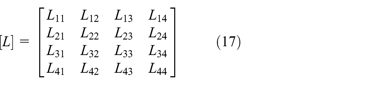
Let [L] = [H]⁻¹, inverse matrix of the matrix [H]

with

$$[L]=\left[\begin{array}{cccc}\hfill L_{11}\hfill & \hfill L_{12}\hfill & \hfill L_{13}\hfill & \hfill L_{14}\hfill \\ \multicolumn{1}{c}{L_{21}}& \hfill L_{22}\hfill & \hfill L_{23}\hfill & \hfill L_{24}\hfill \\ \multicolumn{1}{c}{L_{31}}& \hfill L_{32}\hfill & \hfill L_{33}\hfill & \hfill L_{34}\hfill \\ \multicolumn{1}{c}{L_{41}}& \hfill L_{42}\hfill & \hfill L_{43}\hfill & \hfill L_{44}\hfill \end{array}\right]$$

(17)

Then relation (13) becomes

$$\begin{array}{cc}\multicolumn{1}{c}{}& u(x,y)=[N]\{u\}\hfill \\ \multicolumn{1}{c}{}& [g]=[\begin{array}{cccc}\hfill 1\hfill & \hfill x\hfill & \hfill y\hfill & \hfill \mathrm{xy}\hfill \end{array}]\hfill \end{array}$$

(18)

Interpolation functions {N} in equation (18) are then given by

$$\left\{\begin{array}{c}\hfill N_1(x,y)\hfill \\ \multicolumn{1}{c}{N_2(x,y)}\\ \multicolumn{1}{c}{N_3(x,y)}\\ \multicolumn{1}{c}{N_4(x,y)}\end{array}\right\}=\left\{\begin{array}{c}\hfill L_{11}+L_{12}x+L_{13}y+L_{14}\mathrm{xy}\hfill \\ \multicolumn{1}{c}{L_{21}+L_{22}x+L_{23}y+L_{24}\mathrm{xy}}\\ \multicolumn{1}{c}{L_{31}+L_{32}x+L_{33}y+L_{34}\mathrm{xy}}\\ \multicolumn{1}{c}{L_{41}+L_{42}x+L_{43}y+L_{44}\mathrm{xy}}\end{array}\right\}$$

(19)

Stiffness matrix of a quadrilateral element

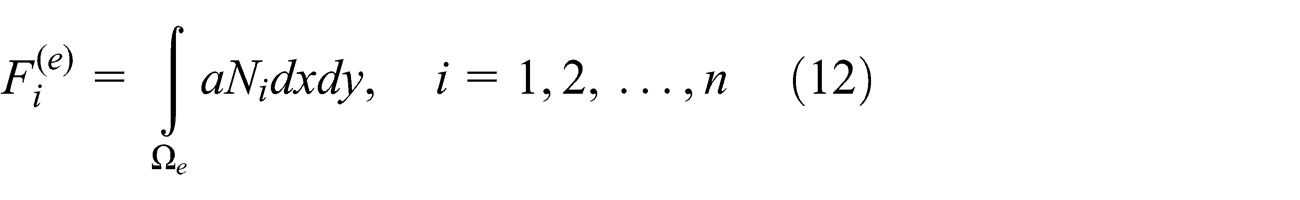
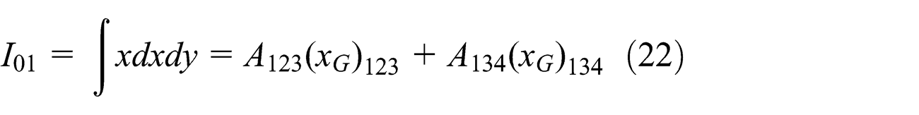
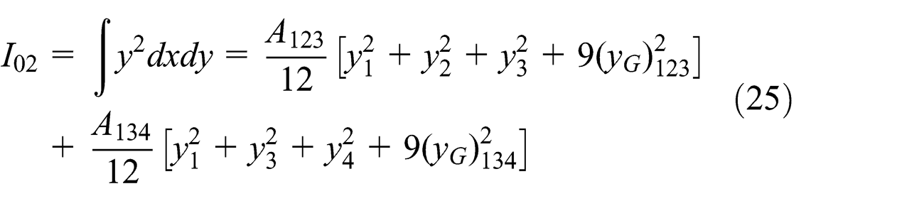
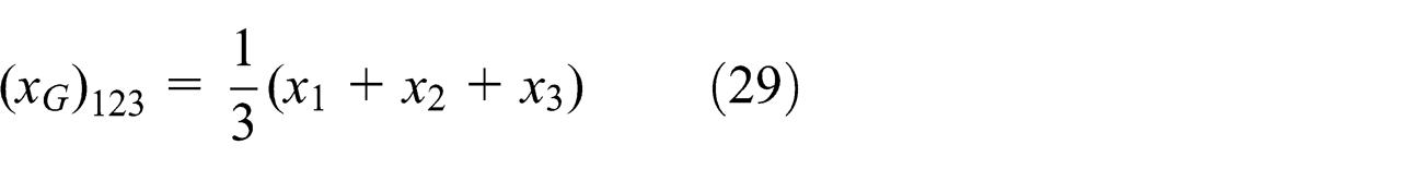
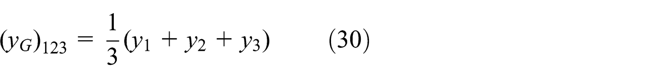
The calculation of the matrices [K ^(e)] and the force vector {F ^(e)} of the element in equation (11) is done by replacing relation (20) in expressions (11) and (13) and then making a direct integration using the results given by relation (20) for a quadrilateral explained below. The quadrilateral element is considered as the union of two triangles as shown in Figure 2. This consideration is made only to calculate the integrals I ₀₀, I ₁₀, I ₀₁, I ₁₁, I ₂₀, I ₀₂, and x_G , y_G of a quadrilateral.

The relations for I_mn (m = 0, 1, 2), (n = 0, 1, 2) in equation (20) and the values of x_G and y_G of any triangle shown as number (1) in Figure 2 are presented in Zienkiewicz et al. ⁴ and Reddy ⁵

$$I_{\mathrm{mn}}=\underset{\Delta }{\int }{x}^m{y}^n\mathrm{dxdy}(m=0,1,2)(n=0,1,2)$$

(20)

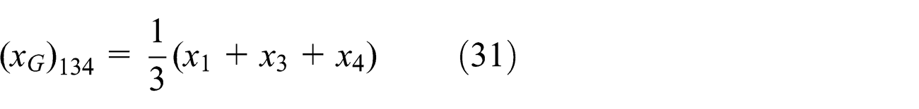
Using these relations, we can calculate the integrals and the position x_G , y_G center of gravity of the quadrilateral element as follows

$$I_{00}=\int \mathrm{dxdy}=A=A_{123}+A_{134}$$

(21)

$$I_{01}=\int \mathrm{xdxdy}=A_{123}{(x_G)}_{123}+A_{134}{(x_G)}_{134}$$

(22)

$$I_{10}=\int \mathrm{ydxdy}=A_{123}{(y_G)}_{123}+A_{134}{(y_G)}_{134}$$

(23)

$$\begin{array}{cc}\multicolumn{1}{c}{I_{20}}& =\int x^2\mathrm{dxdy}=\frac{A_{123}}{12}[x_1^2+x_2^2+x_3^2+9{(x_G)}_{123}^2]\hfill \\ \multicolumn{1}{c}{}& +\frac{A_{134}}{12}[x_1^2+x_3^2+x_4^2+9{(x_G)}_{134}^2]\hfill \end{array}$$

(24)

$$\begin{array}{cc}\multicolumn{1}{c}{I_{02}}& =\int y^2\mathrm{dxdy}=\frac{A_{123}}{12}[y_1^2+y_2^2+y_3^2+9{(y_G)}_{123}^2]\hfill \\ \multicolumn{1}{c}{}& +\frac{A_{134}}{12}[y_1^2+y_3^2+y_4^2+9{(y_G)}_{134}^2]\hfill \end{array}$$

(25)

$$\begin{array}{cc}\multicolumn{1}{c}{I_{11}}& =\int \mathrm{xydxdy}\hfill \\ \multicolumn{1}{c}{}& =\frac{A_{123}}{12}[{\displaystyle \sum _{j=1}^{j=3}}{x}_j{y}_j+9{(x_G)}_{123}{(y_G)}_{123}]\hfill \\ \multicolumn{1}{c}{}& +\frac{A_{134}}{12}[x_1{y}_1+x_3{y}_3+x_4{y}_4+9{(x_G)}_{134}{(y_G)}_{134}]\hfill \end{array}$$

(26)

$$x_G=\frac{A_{123}{(x_G)}_{123}+A_{134}{(x_G)}_{134}}{A}$$

(27)

$$y_G=\frac{A_{123}{(y_G)}_{123}+A_{134}{(y_G)}_{134}}{A}$$

(28)

where ${(x_G)}_{123},{(y_G)}_{123}$ represent the coordinates of the center of gravity of the triangle bounded by nodes 1, 2, and 3, given by

$${(x_G)}_{123}=\frac{1}{3}(x_1+x_2+x_3)$$

(29)

$${(y_G)}_{123}=\frac{1}{3}(y_1+y_2+y_3)$$

(30)

and ${(x_G)}_{134},{(y_G)}_{134}$ present the coordinates of the center of gravity of the triangle bounded by nodes 1, 3, and 4 given by

$${(x_G)}_{134}=\frac{1}{3}(x_1+x_3+x_4)$$

(31)

$${(y_G)}_{134}=\frac{1}{3}(y_1+y_3+y_4)$$

(32)

$A_{123},A_{134}$ have the surface areas of the triangles limited by the respective nodes 1, 2, 3 and 1, 3, 4 as shown in Figure 2, given by

$$A_{123}=\frac{1}{2}[(x_2-x_1)(y_3-y_1)-(y_2-y_1)(x_3-x_1)]$$

(33)

$$A_{134}=\frac{1}{2}[(x_3-x_1)(y_4-y_1)-(y_3-y_1)(x_4-x_1)]$$

(34)

The polar moment of inertia I_P of a quadrilateral is therefore equal to the sum of the moments of inertia with respect to axes x and y passing through the center of gravity of the section. In this case, we should use the formula to allow Huygens transform quadratic moments of inertia of any axis to an axis passing through the center of gravity of the section.

In equation (7), the torsional constant C is equal to the polar moment of inertia I_P for a circular section and different for a non-circular section.

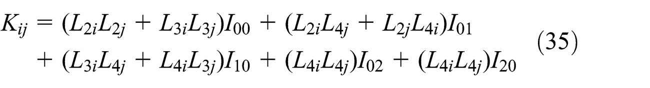
Using equations (11) and (12), with the functions of interpolation (19) and after integration by using expressions (21)–(26), we have the following results

$$\begin{array}{cc}\multicolumn{1}{c}{K_{\mathrm{ij}}}& =(L_{2i}{L}_{2j}+L_{3i}{L}_{3j})I_{00}+(L_{2i}{L}_{4j}+L_{2j}{L}_{4i})I_{01}\hfill \\ \multicolumn{1}{c}{}& +(L_{3i}{L}_{4j}+L_{4i}{L}_{3j})I_{10}+(L_{4i}{L}_{4j})I_{02}+(L_{4i}{L}_{4j})I_{20}\hfill \end{array}$$

(35)

$$F_i^{(e)}=L_{i1}+I_{00}+L_{i2}{I}_{10}+L_{i3}{I}_{01}+L_{i4}{I}_{11}$$

(36)

The stiffness matrix of a quadrilateral element has rank 4 × 4 and the force vector has rank 4. For the finite element, we will have the following matrix form

$$\left[\begin{array}{cccc}\hfill K_{11}\hfill & \hfill K_{12}\hfill & \hfill K_{13}\hfill & \hfill K_{14}\hfill \\ \multicolumn{1}{c}{}& \hfill K_{22}\hfill & \hfill K_{23}\hfill & \hfill K_{24}\hfill \\ \multicolumn{1}{c}{\mathrm{Sym}}& \hfill \hfill & \hfill K_{33}\hfill & \hfill K_{34}\hfill \\ \multicolumn{1}{c}{}& \hfill \hfill & \hfill \hfill & \hfill K_{44}\hfill \end{array}\right]\left\{\begin{array}{c}\hfill u_1\hfill \\ \multicolumn{1}{c}{u_2}\\ \multicolumn{1}{c}{u_3}\\ \multicolumn{1}{c}{u_4}\end{array}\right\}=\left\{\begin{array}{c}\hfill F_1\hfill \\ \multicolumn{1}{c}{F_2}\\ \multicolumn{1}{c}{F_3}\\ \multicolumn{1}{c}{F_4}\end{array}\right\}$$

(37)

The elemental stiffness matrix is singular. We note that the elemental stiffness matrix must be singular.

A problem is encountered during the determination of the coefficients of the stiffness matrix. This is the calculation of the matrix [L] as the inverse of the matrix [H] for each finite element mesh. Since the rank of this matrix is small (equal to 4), the problem is reduced. For information, the number of mathematical operations that makes the inversion procedure of a matrix of order 4 × 4 is about 300 operations.^4,20,21

Assembly of elementary stiffness matrices

The assembly is the operation which consists in building the global matrix [K] and global vector {F} for the entire domain from the elementary matrices [K ^(e)] and elementary vectors {f ^(e)} of the finite elements. To represent the assembly of finite element matrices, we illustrate the procedure considering that the mesh is built by two quadrilaterals.

$[K_{\mathrm{ij}}^{(1)}]$ and $[K_{\mathrm{ij}}^{(2)}]$ (i, j = 1, 2, 3, 4) are the coefficients of the stiffness matrices corresponding to the two elements and $\{F_i^{(1)}\}$ and $\{F_i^{(2)}\}$ (i = 1, 2, 3, 4) are the cases of the force vector of the two elements, respectively. The finite element mesh is shown in Figure 3.

Figure 3.

Assembling two quadrilateral elements.

From this mesh, we note the correspondence between the global values and the nodal values of the elements^4,5

$$\begin{array}{c}\multicolumn{1}{c}{u_1=u_1^{(1)},u_2=u_4^{(1)},u_3=u_2^{(1)}=u_1^{(2)}}\\ \multicolumn{1}{c}{u_4=u_3^{(1)}=u_4^{(2)},u_5=u_2^{(2)},u_6=u_3^{(2)}}\end{array}$$

(38)

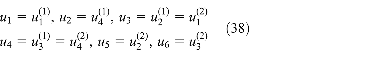
For element (1), one has:

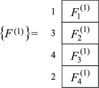
For element (2), we have:

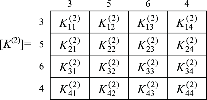
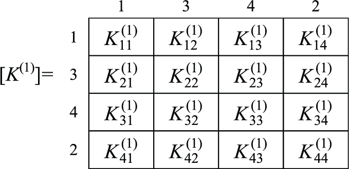
Outside the stiffness matrices and vectors elemental of elements (1) and (2), we see numbers (1, 3, 4, and 2) for element (1) and numbers (3, 5, 6, and 4) for element (2) in this order as shown in Figure 3.

These numbers correspond to the location of the boxes in each matrix and vector in the global stiffness matrix and force vector. So for the entire domain, we have the following result

$$[K]=\left[\begin{array}{cccccc}\hfill K_{11}^{(1)}\hfill & \hfill K_{14}^{(1)}\hfill & \hfill K_{12}^{(1)}\hfill & \hfill K_{13}^{(1)}\hfill & \hfill 0\hfill & \hfill 0\hfill \\ \multicolumn{1}{c}{K_{41}^{(1)}}& \hfill K_{44}^{(1)}\hfill & \hfill K_{32}^{(1)}\hfill & \hfill K_{43}^{(1)}\hfill & \hfill 0\hfill & \hfill 0\hfill \\ \multicolumn{1}{c}{K_{21}^{(1)}}& \hfill K_{32}^{(1)}\hfill & \hfill K_{22}^{(1)}+K_{11}^{(2)}\hfill & \hfill K_{24}^{(1)}+K_{14}^{(2)}\hfill & \hfill K_{12}^{(2)}\hfill & \hfill K_{13}^{(2)}\hfill \\ \multicolumn{1}{c}{K_{31}^{(1)}}& \hfill K_{34}^{(1)}\hfill & \hfill K_{32}^{(1)}+K_{41}^{(2)}\hfill & \hfill K_{33}^{(1)}+K_{44}^{(2)}\hfill & \hfill K_{42}^{(2)}\hfill & \hfill K_{43}^{(2)}\hfill \\ \multicolumn{1}{c}{0}& \hfill 0\hfill & \hfill K_{21}^{(2)}\hfill & \hfill K_{24}^{(2)}\hfill & \hfill K_{22}^{(2)}\hfill & \hfill K_{23}^{(2)}\hfill \\ \multicolumn{1}{c}{0}& \hfill 0\hfill & \hfill K_{31}^{(2)}\hfill & \hfill K_{34}^{(2)}\hfill & \hfill K_{32}^{(2)}\hfill & \hfill K_{33}^{(2)}\hfill \end{array}\right]$$

(39)

$$\left\{F\right\}=\left\{\begin{array}{c}\hfill F_1^{(1)}\hfill \\ \multicolumn{1}{c}{F_3^{(1)}}\\ \multicolumn{1}{c}{F_4^{(1)}+F_1^{(2)}}\\ \multicolumn{1}{c}{F_2^{(1)}+F_4^{(2)}}\\ \multicolumn{1}{c}{F_2^{(2)}}\\ \multicolumn{1}{c}{F_3^{(2)}}\end{array}\right\}$$

(40)

Matrix (39) is the global stiffness matrix of the entire domain. It is of rank 6 × 6, as the number of nodes in the domain is equal to 6. We note here that each node contains a single degree of freedom (an unknown). Equation (40) represents the force vector of the entire domain. It is of rank 6.

Grid generation

The implementation of the finite element method requires the use of the powerful numerical methods to solve the algebraic system which results from it. These equations will be solved in a discrete field, while passing from a medium continues in a discretized medium. In this paragraph, one deals with the problem of grid generation for the 2D fields.^4,9,19 Therefore, one will develop an algebraic method that gives a structured grid, whose cells are of form quadrilaterals. It is named as standard grid “H.”

Procedure of grid generation

We are interested in the 2D simply connected domain. The general form is represented in Figure 4. To generate the grid inside this domain, and among the several existing techniques and according to the method of resolution of the algebraic system of equation, as well as the manner of consideration of the shape of the matrix of rigidity, it is very interesting to apply the idea of generation of grid in the rectangular areas for this type of problem.

Figure 4.

Boundary of a simply connected domain.

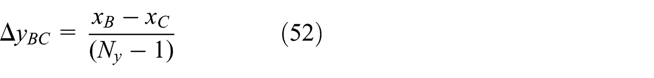
Therefore, we obtain four sides which are AD, AB, BC, and CD, respectively. If we make continuous changes in each side, one can render lines straight. Consider the subdivision by N_x and N_y nodes on the horizontal x-axis and vertical y-axis, respectively.

Generation of nodes on the boundary of the domain

In the general case, it is not easy to make a universal method that will be applied for any curves, but we try to adapt to each complex forms a suitable procedure. The choice of points A, B, C, and D affects the shape of the four sides of the domain.

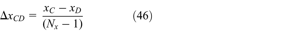
Consider the sides AB and CD. We look at what divides the segment [x_A , x_B ] in N_x nodes, then determine y_i (i = 1, 2, …, N_x ) or the corresponding to divide the segment [y_A , y_B ] in N_x nodes, and then determine x_i (i = 1, 2, …, N_x ). To take decisions, we try to calculate the following values

$$x_{\mathrm{dis}}=|x_B-x_A|;y_{\mathrm{dis}}=|y_B-y_A|$$

(41)

One makes calculation between the maximum value of x_dis and y_dis by

$$d_{max}=\mathrm{Max}(x_{\mathrm{dis}},y_{\mathrm{dis}})$$

(42)

If d_max  = x_dis , we propose the values of x_i (i = 1, 2, …, N_x ) and then determine y_i using the function that passes through points A and B. It is assumed that in fact the choice of x_i then calculate y_i . Then the segment [x_A , x_B ] is divided into N_x nodes with points A and B included. For simplicity, we chose a subdivision not constant, and if the side is curved in the vicinity of point A or B, or any area, it is recommended to use a condensation process node, the procedure of which will be presented in the next section. $(N_x-1)$ subintervals are thus obtained. The length of each interval is given by

$$\Delta x_{\mathrm{AB}}=\frac{|x_B-x_A|}{(N_x-1)}$$

(43)

The coordinates of the points on this side are given by

$$x_{\mathrm{AB}}(i)=x_A+(i-1)\Delta x_{\mathrm{AB}},i=1,2,\dots ,N_x$$

(44)

$$y_{\mathrm{AB}}(i)=f_{\mathrm{AB}}(x_{\mathrm{AB}}(i)),i=1,2,\dots ,N_x$$

(45)

For the CD side, and by analogy with the AB side, we have the following results

$$\Delta x_{\mathrm{CD}}=\frac{x_C-x_D}{(N_x-1)}$$

(46)

$$x_{\mathrm{DC}}(i)=x_D+(i-1)\Delta x_{\mathrm{CD}},i=1,2,\dots ,N_x$$

(47)

$$y_{\mathrm{DC}}(i)=f_{\mathrm{DC}}(x_{\mathrm{DC}}(i)),i=1,2,\dots ,N_x$$

(48)

where F_DC (x) is the function of the side DC.

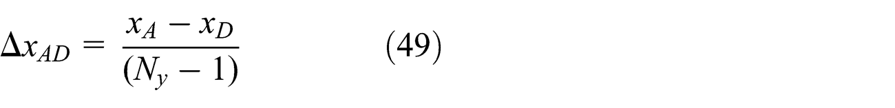
The generation of hard node edges AD and BC is the same approach as the sides AB and DC. We will have for the AD side

$$\Delta x_{\mathrm{AD}}=\frac{x_A-x_D}{(N_y-1)}$$

(49)

$$x_{\mathrm{AD}}(i)=x_D+(j-1)\Delta x_{\mathrm{DC}},j=1,2,\dots ,N_y$$

(50)

$$y_{\mathrm{AD}}(i)=f_{\mathrm{AD}}(x_{\mathrm{AD}}(i)),j=1,2,\dots ,N_y$$

(51)

For the side BC, we have

$$\Delta y_{\mathrm{BC}}=\frac{x_B-x_C}{(N_y-1)}$$

(52)

$$x_{\mathrm{BC}}(j)=x_C+(j-1)\Delta y_{\mathrm{BC}},j=1,2,\dots ,N_y$$

(53)

$$y_{\mathrm{BC}}(j)=f_{\mathrm{BC}}(x_{\mathrm{BC}}(j)),j=1,2,\dots ,N_y$$

(54)

Finally, we obtain a diagram as presented in Figure 5. The example shown is for N_x  = 10 and N_y  = 6.

Figure 5.

Nodes’ generation on the boundary of the domain.

Stretching function

The stretching function is used for one-dimensional (1D) distributed point along a boundary area where the area requires a specific resolution. In this case, the gradient of the solution is high.^4,22

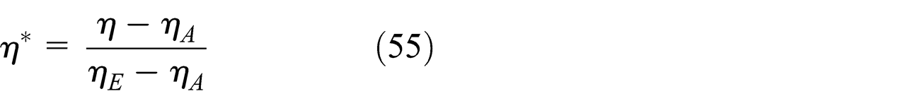
If the stretching function is applied to the side EA in Figure 6, the normalized variable is given by

$${\eta }^{*}=\frac{\eta -{\eta }_A}{{\eta }_E-{\eta }_A}$$

(55)

Figure 6.

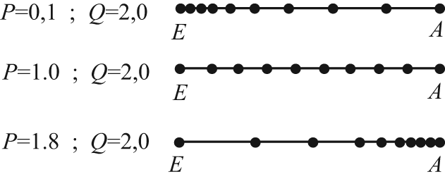
Distribution of nodes according to equation (56).

with $0\le {\eta }^{*}\le 1\mathrm{and}{\eta }_A\le \eta \le {\eta }_E$

where η represents x or y.

We can even give the distribution on the interval [0, 1] by η^* with equal subintervals. The used stretching function is given by^4,22

$$s=P{\eta }^{*}+(1-P)[1-\frac{\tanh [Q(1-{\eta }^{*})]}{\tanh [Q]}]$$

(56)

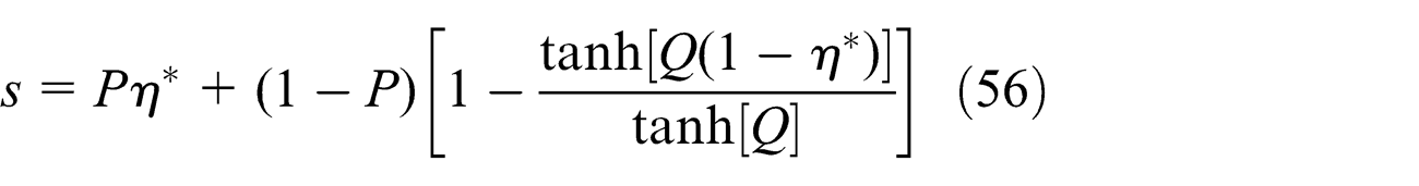
Once the value of s is obtained, it is required to specify the distribution of x and y. For example

$$x=x_A+s(x_A-x_E),y=y_A+s(y_A-y_E)$$

(57)

For values of P > 1.0, it is possible to condense the nodes to point A.

Typical distributions of points on the EA segment for different values of P and Q are shown in Figure 6.

Generation of internal nodes

We now proceed with the presentation of the method used for the generation of internal nodes. The procedure involves first to determine the x-abscissa x_i of all points by ignoring the order and by interpolating between the left and right sides (see Figure 7). We proceed by following the determination of ordinates y_i of these nodes by interpolation between the top and bottom sides of the domain (see Figure 8). We follow the same approach presented for the generation of boundary points. Details of the procedure are given in Zienkiewicz et al. ⁴

Figure 7.

Illustration of the procedure for determining the abscissa.

Figure 8.

Illustration of the procedure for determining the ordinates.

Numbering of nodes

The numbering of nodes plays a very important role in the storage of matrices, especially if the rank of the matrix becomes higher.^4,14–16 For any order N × N of matrix, it is necessary to store N ² boxes, which is impossible for high values of N. The need for computer memory is important for our problem, which forces us to think of a technique to solve a high-order system of equations, to make the resolution of the physical problem with good required precision. ⁴

If we look at the field, we can make the stiffness matrix full of zero which condenses to a known region and the non-zero elements to condense the main diagonal of the matrix. This is called as band matrices.^4,10–16 In addition, the mathematical formulation by finite element gives a symmetric matrix.

The result of the application of mathematical operations between two real numbers, one of which is 0, is known to start again without a computer calculation. So, there is no need to book a whole box to store a 0. As the number of zeros may be important, it remains to indicate their positions in the stiffness matrix. This matrix is characterized by the value of the half-bandwidth. The number of zeros in the matrix increases as the value of the half-bandwidth decreases. ⁴

It should be noted that one can find the band of the zero elements. But if we want to work with band matrices, we cannot eliminate these items from the store because working with this type of matrix and the decomposition into two triangular matrices is also band. Note that if we calculate the number of zeros that are in the band part, we can find some numbers to a number that exceeds half or even 90%. ⁴

The width of the half-band is equal to the maximum difference one (problem intervals) between the numbers of two nodes of the same element, multiplied by the number of degrees of freedom of the nodes (in our case, each node contains 1 degree of freedom). If we have a rectangular area formed by NE quadrilateral elements, the value of the half-band B of the matrix before applying the boundary conditions is given by (Figure 9).

Figure 9.

Finite element quadrilateral with four nodes.

Let $B_L$ be the value of the half-band given by the element number L. Then

$$B_L=\mathrm{Max}(i_1,i_2,i_3,i_4)-\mathrm{Min}(i_1,i_2,i_3,i_4)+1$$

(58)

Therefore, the value of B is given by

$$B=\mathrm{Max}(B_1,B_2,B_3,\dots ,B_{\mathrm{NE}})$$

(59)

Consider a rectangular area to be discretized in 15 quadrilaterals as shown in the following figure elements (Figure 10).

Figure 10.

Elements’ numbering.

The numbering of the elements is not a problem on the value of the half-band of the stiffness matrix. Both numbering nodes are considered for this example. For each case, we will build the stiffness matrix of the whole area and that regardless of the boundary conditions. It should be noted that for this example, the number of nodes is 24, then the stiffness matrix [K] is of rank (24 × 24).

Case 1

We will number the nodes along the horizontal axis from left to right and climb along the vertical y-axis as shown in Figure 11.

Figure 11.

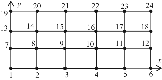
Example of numbering of nodes (case 1).

We found in this case B = 8.

Case 2

We will now number the nodes along the vertical y-axis from the bottom to the top and then move along the horizontal x-axis from left to right (see Figure 12).

Figure 12.

Example of numbering of nodes (case 2).

It may be noted in this case that the width of the half-band equals B = 6. We deduce from both numbering as case 2 is an optimal numbering for which the non-zero cells condense as much as possible to the main diagonal.

Node filtering

Sometimes it is very efficient to use the filter option called nodes. In some cases, the size of grid cells is not homogeneous. There is a large cell size and other very small. Especially, for points close to the boundary. To make the cell sizes of same magnitude, it repositions the internal mesh points several times using the procedure described by the following equation (60) ⁴

$$\begin{array}{c}\multicolumn{1}{c}{x_i^{\mathrm{new}}=x_i^{\mathrm{old}}-\frac{\omega }{m}{\displaystyle \sum _{k=1}^{k=m}}(x_k^{\mathrm{old}}-x_i^{\mathrm{old}})}\\ \multicolumn{1}{c}{y_i^{\mathrm{new}}=y_i^{\mathrm{old}}-\frac{\omega }{m}{\displaystyle \sum _{k=1}^{k=m}}(y_k^{\mathrm{old}}-y_i^{\mathrm{old}})}\end{array}$$

(60)

Connection of the finite element mesh

According to the discretization of the domain into small elements, we obtain a set of points and finite elements. Each element has its own stiffness matrix [K ^(e)] and force vector {f ^(e)}. The problem is to assemble these elementary matrices for the entire domain. To get results, we have to know the numbers of nodes of each element. So, we must declare a matrix of order (NE × 4). We denote this matrix by NUMNT. For example, both previous numbering, the vector NUMNT (NE, 4), will be filled as follows:

The four values in each row of the vector NUMNT represent the numbers of rows and columns of the matrix of the overall stiffness matrix before applying boundary conditions.

Preparation of the system of equations

In this section, we will present the necessary steps and the technique developed for the preparation of the system of algebraic equations. More precisely, the stiffness matrix [K] of the overall matrix and the force vector {f} correspond. Our problem here is to prepare the system of equations before and after the introduction of the boundary conditions, in addition, as a vector. ⁴

The rank of the stiffness matrix of the system before the introduction of the boundary conditions is equal to NN, and after the introduction of the boundary conditions becomes number of remaining degree of freedom (NDDLR), less than NN, which will be reduced by number of eliminated degree of freedom (NDDLE). We note here that the stiffness matrix is singular and that before the introduction of the boundary conditions removes the singularity of the matrix and makes it regular. The problem here is that the numbers of rows and columns removed in the stiffness matrix before introducing the boundary conditions during the phase of implementation of these are the numbers of nodes in the border area. To get to the removal of these rows and columns, we must declare a vector of integer type, of rank NN, named, for example, ICL, to indicate each domain node by its presence or absence in the final stiffness matrix by a code. The code used here are the two digits 0 and 1.

• If ICL(I) = 1, then the node number “I” will be present in the final matrix.

• If ICL(I) = 0, then the node number “I” is absent in the final matrix.

Can be drawn from this filling, the number of boxes containing “1” is the same for both cases and is equal to 8 for these examples. This number is the rank of the final stiffness matrix after the application of boundary conditions.

After we did the filling of the vector “ICL,” where the knowledge of rows and columns was removed from the stiffness matrix after the introduction of boundary conditions, we have to know otherwise. That is to say, the number of node in the mesh corresponding to the row or column of the final stiffness matrix. The form of the stiffness matrix of the two cases’ numbering after the introduction of boundary conditions has the following form, and that after removing the rows and columns with the numbers of nodes in the border area. The rank of the matrix is (8 × 8). We can look exactly the numbers of lines remaining as columns as presented in Figure 13.

Figure 13.

Forms of the matrix [K] of the two cases’ numbering after application of boundary conditions.

If we do a little comparison in the change of the value of B in case 1 and case 2, we note that the value of B is changed. It decreases or remains the same. For case 1, the new value becomes 6. For case 2, it becomes 4.

Numerical solution of system of algebraic equations

This section is devoted to solving the problem numerically. We implemented a program in FORTRAN language in this context. The work was limited to symmetric band matrices [K]. These two properties led us to store the upper (or lower) of the matrix, by eliminating the zeros which are on the outside of the band, in a single-column vector, which gives the equivalence of boxes for matrix [K] in the vector {vk}.

The calculation is simple and it is to give every time we fall into a cell of the matrix K(i, j), its position in the vector {vk} from a certain recurrence formula that varies with the way storage. If once we fall into a K(i, j) box above the diagonal (at the top) but outside of the band, the calculation will be ignored as this box is actually 0 and it has no change statement. If once we fall into a K(i, j) box below the diagonal (in the bottom), it is sufficient to use only the property K(i, j) = K (j, i) (storing the upper part was chosen in the program), and the treatment is as a K(i, j) with the two previous cases.

Methods of storing a matrix as a vector

Consider a matrix [K] of order (N × N) symmetric and band. The problem is how to store the boxes of the matrix band in a vector {vk}. We propose in our work is the storage as diagonal. The principle is presented as follows. We take a matrix [K] of order (7 × 7) and symmetric and the bandwidth B = 4 and that for fixed ideas. ⁴

The method chosen storage is represented by the direction of the arrows, that is to say, diagonal by diagonal, as shown in Figure 14.

Figure 14.

Diagonal storage.

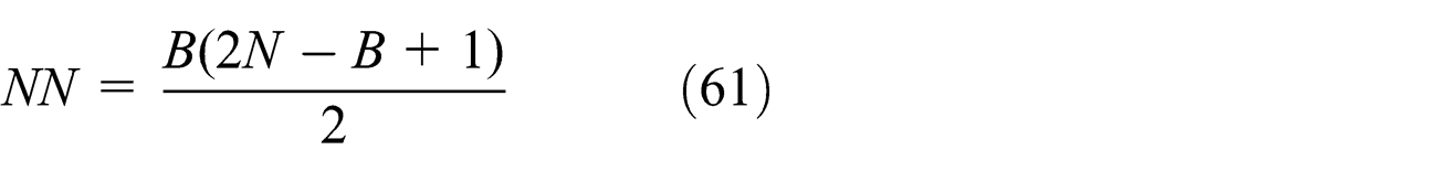
It may be noted in this example that the required dimension of the vector {vk} is equal to NN = 22. Now, if we want to generalize for matrix [K] of order (N × N) symmetric with width of half-band B, we have

$$\mathrm{NN}=\frac{B(2N-B+1)}{2}$$

(61)

We now proceed to the determination of the storage formula of the matrix elements [K] (the elements of the upper band only) in the vector {vk}, that is to say, the equivalent of a box of the matrix [K] in the vector {vk}.

For boxes K(i, j), its position in the vector {vk} is (L) with

$$L={\displaystyle \sum _{p=1}^{p=j-i}}(N+1-P)+i=\frac{1}{2}(j-i)(2N-j+i+1)+i$$

(62)

where $\{\begin{array}{c}\hfill j=1,2,3,\dots ,B\hfill \\ \multicolumn{1}{c}{i=j,2,3,\dots ,B}\end{array}\mathrm{and}\{\begin{array}{c}\hfill j=B+1,B+2,\dots ,N\hfill \\ \multicolumn{1}{c}{i=j-B,j-B+1,\dots ,j}\end{array}$

The method of storage of matrix band vector form saves us in memory in the following order

$$\mathrm{NDCE}=N^2-\mathrm{NN}=N^2-\frac{B(2N-B+1)}{2}$$

(63)

Instead of storing N ² cases, it only stores NN boxes. For an order of values NDCE and NN, we propose the following example:

• N = 100

B	N 2	NN	NDCE	Cases won (%)
100	10,000	5050	4950	49.50
70	10,000	4585	5415	54.15
35	10,000	2905	7095	70.95
10	10,000	955	9045	90.45
2	10,000	199	9801	98.01

It is clear from this example that more than half the width of the band is smaller than the number of cases increasing rapidly.

Algorithm for solving the system of equations

It is necessary to solve the problem, after completing the stiffness matrix [K] and the global vector {F}, to determine the vector {u} solution to the following system of equations^{4,10–13,20,21}

$$[K]\{u\}=\{F\}$$

(64)

We chose the method of direct numerical solution of Khaletski. ⁴ For a symmetric band matrix, the algorithm for solving system (64) is presented in Zienkiewicz et al. ⁴ Let the matrix [K] as a product of two lower triangular matrices [L] = [L_ij ] and the upper triangular matrix [H] = [H_ij ] have unit diagonal, that is to say

$$[K]=[L][H]$$

(65)

It will result in two systems of equations with a triangular matrix

$$[K]\{u\}=\{F\}\to [L][H]=\{f\}$$

we put

$$[H]\{u\}=\{y\}$$

(66)

then

$$[L]\{y\}=\{F\}$$

(67)

If the matrix [K] is symmetric, we can show that

$$H_{\mathrm{ij}}=\frac{L_{\mathrm{ji}}}{L_{\mathrm{ii}}}$$

(68)

The matrix [K] has the following general form

$$\left[\begin{array}{cccccccccc}\hfill K_{11}\hfill & \hfill \hfill & \hfill \hfill & \hfill \hfill & \hfill \hfill & \hfill \hfill & \hfill \hfill & \hfill \hfill & \hfill \hfill & \hfill \hfill \\ \multicolumn{1}{c}{K_{21}}& \hfill K_{22}\hfill & \hfill \hfill & \hfill \hfill & \hfill \hfill & \hfill \hfill & \hfill \hfill & \hfill \hfill & \hfill \hfill & \hfill \hfill \\ \multicolumn{1}{c}{K_{31}}& \hfill K_{32}\hfill & \hfill \hfill & \hfill \hfill & \hfill \hfill & \hfill \hfill & \hfill \hfill & \hfill \hfill & \hfill \hfill & \hfill \hfill \\ \multicolumn{1}{c}{⋮}& \hfill ⋮\hfill & \hfill \hfill & \hfill \ddots \hfill & \hfill \hfill & \hfill \hfill & \hfill \mathrm{Sym}\hfill & \hfill \hfill & \hfill \hfill & \hfill \hfill \\ \multicolumn{1}{c}{K_{B1}}& \hfill K_{B2}\hfill & \hfill ⋮\hfill & \hfill \hfill & \hfill \ddots \hfill & \hfill \hfill & \hfill \hfill & \hfill \hfill & \hfill \hfill & \hfill \hfill \\ \multicolumn{1}{c}{0}& \hfill K_{B+1,2}\hfill & \hfill ⋮\hfill & \hfill \hfill & \hfill \hfill & \hfill \ddots \hfill & \hfill \hfill & \hfill \hfill & \hfill \hfill & \hfill \hfill \\ \multicolumn{1}{c}{}& \hfill 0\hfill & \hfill \hfill & \hfill \hfill & \hfill \hfill & \hfill \hfill & \hfill K_{\mathrm{ii}}\hfill & \hfill \hfill & \hfill \hfill & \hfill \hfill \\ \multicolumn{1}{c}{⋮}& \hfill ⋮\hfill & \hfill ⋮\hfill & \hfill \hfill & \hfill \ddots \hfill & \hfill \begin{array}{c}\hfill \hfill \\ \multicolumn{1}{c}{}\end{array}\hfill & \hfill \begin{array}{c}\hfill ⋮\hfill \\ \multicolumn{1}{c}{⋮}\end{array}\hfill & \hfill \begin{array}{c}\hfill \hfill \\ \multicolumn{1}{c}{\ddots }\end{array}\hfill & \hfill \hfill & \hfill \hfill \\ \multicolumn{1}{c}{}& \hfill \hfill & \hfill \hfill & \hfill \hfill & \hfill \hfill & \hfill \hfill & \hfill \begin{array}{c}\hfill K_{B+i-1,i}\hfill \\ \multicolumn{1}{c}{⋮}\end{array}\hfill & \hfill \hfill & \hfill \ddots \hfill & \hfill \hfill \\ \multicolumn{1}{c}{0}& \hfill 0\hfill & \hfill 0\hfill & \hfill \hfill & \hfill \cdots \hfill & \hfill \hfill & \hfill 0\hfill & \hfill \hfill & \hfill \hfill & \hfill K_{\mathrm{NN}}\hfill \end{array}\right]$$

(69)

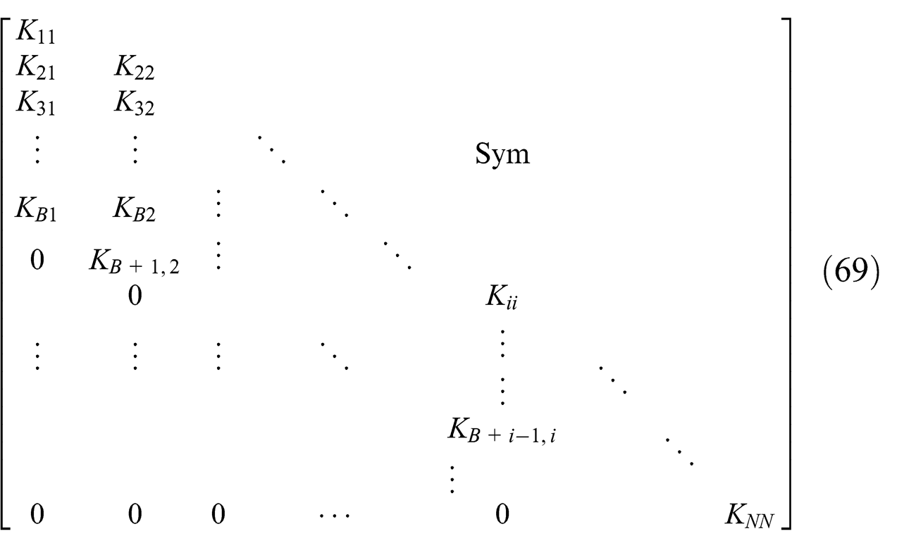
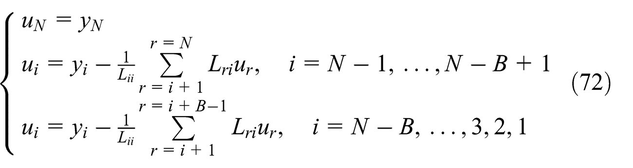
The matrix [L], which belongs to the decomposition of the matrix [K], has the same structure as [K] except that it is triangular. After removal operations on zeros (the external elements of the band), the elements of the matrix [L] can be calculated by the following equations ⁴

$$\{\begin{array}{c}\hfill L_{\mathrm{ij}}=K_{\mathrm{ij}}-{\displaystyle \sum _{r=1}^{r=j-1}}{L}_{\mathrm{ir}}\frac{L_{\mathrm{jr}}}{L_{\mathrm{rr}}}\{\begin{array}{c}\hfill i=1,2,\dots ,B\hfill \\ \multicolumn{1}{c}{j=2,3,\dots ,i}\end{array}\hfill \\ \multicolumn{1}{c}{L_{\mathrm{ij}}=K_{\mathrm{ij}}-{\displaystyle \sum _{r=i-B+1}^{r=j-1}}{L}_{\mathrm{ir}}\frac{L_{\mathrm{jr}}}{L_{\mathrm{rr}}}\{\begin{array}{c}\hfill i=B+1,\dots ,N\hfill \\ \multicolumn{1}{c}{j=i-B+1,\dots ,i}\end{array}}\end{array}$$

(70)

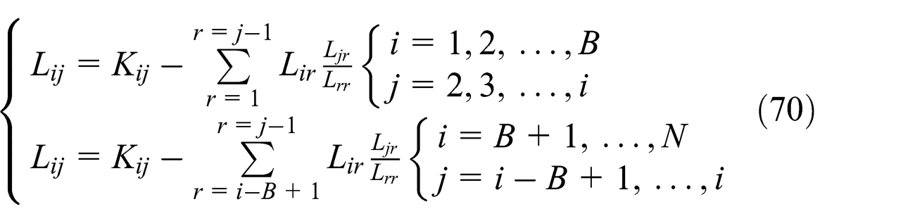
Similarly, the vector {y} from equation (67) and the vector {u} from equation (66) can be calculated by the following algorithm ⁴

$$\{\begin{array}{c}\hfill y_1=\frac{F_1}{L_{11}}\hfill \\ \multicolumn{1}{c}{y_i=\frac{1}{L_{\mathrm{ii}}}(F_i-{\displaystyle \sum _{r=1}^{r=i-1}}{L}_{\mathrm{ir}}{y}_r),i=2,3,\dots ,B}\\ \multicolumn{1}{c}{y_i=\frac{1}{L_{\mathrm{ii}}}(F_i-{\displaystyle \sum _{r=i-B+1}^{r=i-1}}{L}_{\mathrm{ir}}{y}_r),i=B+1,\dots ,N}\end{array}$$

(71)

and

$$\{\begin{array}{c}\hfill u_N=y_N\hfill \\ \multicolumn{1}{c}{u_i=y_i-\frac{1}{L_{\mathrm{ii}}}{\displaystyle \sum _{r=i+1}^{r=N}}{L}_{\mathrm{ri}}{u}_r,i=N-1,\dots ,N-B+1}\\ \multicolumn{1}{c}{u_i=y_i-\frac{1}{L_{\mathrm{ii}}}{\displaystyle \sum _{r=i+1}^{r=i+B-1}}{L}_{\mathrm{ri}}{u}_r,i=N-B,\dots ,3,2,1}\end{array}$$

(72)

The diagonal elements of the matrix [K] are all positive and non-zero. Similarly, it is a positive definite matrix.

Calculation of parameters of interest

After determining the solution vector {u} in each node of the mesh, our interest is directed toward the computation of some interesting parameters.

The surface area has been divided into small finite elements’ simple quadrilateral shape. Then, the total area of this section will be approximated by the sum of all areas of the surfaces of the finite elements. We can therefore write

$$A={\displaystyle \sum _{i=1}^{i=\mathrm{NE}}}{A}_i$$

(73)

The center of gravity of this section consisting of small quadrilateral element is given by

$$x_G=\frac{{\displaystyle \sum _{i=1}^{i=\mathrm{NE}}}{(x_G)}_i{A}_i}{A};y_G=\frac{{\displaystyle \sum _{i=1}^{i=\mathrm{NE}}}{(y_G)}_i{A}_i}{A}$$

(74)

The polar inertia I_P of the complete section relative to the axis passing through the center of gravity of the section can be calculated by the following equation. Then

$$I_P={\displaystyle \sum _{i=1}^{i=\mathrm{NE}}}{(I_{20})}_i+{\displaystyle \sum _{i=1}^{i=\mathrm{NE}}}{(I_{02})}_i-[{(x_G)}^2+{(y_G)}^2]A$$

(75)

The values of A and x_G and y_G are given by equations (73) and (74), respectively. The expressions of I ₂₀ and I ₀₂ in equation (75) are given by equations (24) and (25), respectively.

Constant of torsion

The calculation of the torsional constant C of the section of the field discretized into NE quadrangles can be calculated using equation (7). We can consider the integral as follows

$$C=4{\displaystyle \sum _{i=1}^{i=\mathrm{NE}}}[\underset{A_i}{\int }u(x,y)\mathrm{dxdy}]$$

(76)

The function u(x, y) of the finite element is given by formula (18) and the interpolation functions are provided by equation (19). Substituting these two equations in equation (76), we have

$$C=4{\displaystyle \sum _{i=1}^{i=\mathrm{NE}}}{\left[\begin{array}{c}\hfill (L_{11}{I}_{00}+L_{21}{I}_{10}+L_{31}{I}_{01}+L_{41}{I}_{11})u_1\hfill \\ \multicolumn{1}{c}{+(L_{12}{I}_{00}+L_{22}{I}_{10}+L_{32}{I}_{01}+L_{42}{I}_{11})u_2}\\ \multicolumn{1}{c}{+(L_{13}{I}_{00}+L_{23}{I}_{10}+L_{33}{I}_{01}+L_{43}{I}_{11})u_3}\\ \multicolumn{1}{c}{+(L_{14}{I}_{00}+L_{24}{I}_{10}+L_{34}{I}_{01}+L_{44}{I}_{11})u_4}\end{array}\right]}_i$$

(77)

Substituting the result obtained by equation (77) in equation (6), we can easily deduce the value of the torsion angle unit.

Stress of torsion

After determining the flow distribution u of twist, the torsional constant C, and unit twist angle θ, we can determine the distribution of torsional stress in both x and y directions for each node of the computational domain using equations (5). Using relations (18) and (19) into equation (5), we have

$${\left(\frac{{\tau }_{\mathrm{xz}}}{M_t}\right)}_i=\frac{2}{C}{\displaystyle \sum _{j=1}^{j=4}}{\left[\begin{array}{c}\hfill (L_{3j}+L_{4j}x)u_1+(L_{3j}+L_{4j}x)u_2\hfill \\ \multicolumn{1}{c}{+(L_{3j}+L_{4j}x)u_3+(L_{3j}+L_{4j}x)u_4}\end{array}\right]}_i$$

(78)

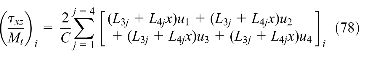
where i = 1, 2, …, NN

$${\left(\frac{{\tau }_{\mathrm{yz}}}{M_t}\right)}_i=\frac{2}{C}{\displaystyle \sum _{j=1}^{j=4}}{\left[\begin{array}{c}\hfill (L_{2j}+L_{4j}y)u_1+(L_{2j}+L_{4j}y)u_2\hfill \\ \multicolumn{1}{c}{(L_{2j}+L_{4j}y)u_3+(L_{2j}+L_{4j}y)u_4}\end{array}\right]}_i$$

(79)

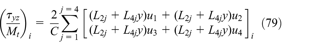
where i = 1, 2, …, NN

For each mesh point, we have two components of torsional stress appointed by τ_xz and τ_yz . The resultant is then given by the following relationship. This constraint works in the section of the beam in the directions well determined

$$\frac{{\tau }_{\mathrm{xs}}}{M_i}=\sqrt{{\left(\frac{{\tau }_{\mathrm{xz}}}{M_t}\right)}^2+{\left(\frac{{\tau }_{\mathrm{yz}}}{M_t}\right)}^2}$$

(80)

It is interesting to determine the value and position of the maximum stress τ of the problem, to locate the dangerous section and the dangerous point which causes the rupture, or to make a design of a working structure under less stress to allowable stress breaking.

The calculation of the relative error made between the exact solution and the approximated numerical solution can be calculated by the following equation

$$\epsilon (\mathrm{\%})=|1-\frac{{\mathrm{Parameter}}_{\mathrm{Computed}}}{{\mathrm{Parameter}}_{\mathrm{Exact}}}|\times 100$$

(81)

The word parameter in equation (81) may indicate the polar moment of inertia, torsional constant, the maximum stress, and all other parameters of the problem.

Results and comments

The first part of the results is to obtain and display the obtained H-type meshes in simple configurations and other complex. The second part is devoted to the presentation of the results on solving the Poisson equation in selected configurations.

Results of the mesh generation

Figure 15 shows a type of quadrilateral mesh in a circular domain. Here, we took an example for N_x  = 30 and N_y  = 30. Therefore, the number of nodes is equal to 900 and the number of quadrilaterals is equal to 841.

Figure 15.

Quadrilateral mesh in a circle with N_x  = 30 and N_y  = 30.

Figures 16–27 present a mesh areas in regular polygons inscribed in a circle, each having a number of sides equal to 3, 4, 5, 6, 7, 8, 9, 10, 11, 12, 13, and 14. In Figure 16, the field is an equilateral triangle. Figure 17 shows a quadrilateral mesh in a square domain. Figure 18 shows a mesh in a pentagon area. The mesh shown in Figures 19–23 is the hexagon, heptagon, octagon, nanogone, and decagon, respectively. Similarly, an area of a regular polygon with 11, 12, 13, and 14 sides were presented in Figures 24–27, respectively.

Figure 16.

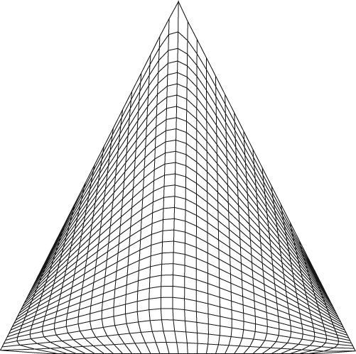
Quadrilateral mesh in an equilateral triangle with N_x  = 30 and N_y  = 30.

Figure 17.

Quadrilateral mesh in a square with N_x  = 20 and N_y  = 20.

Figure 18.

Quadrilateral mesh in a regular pentagon with N_x  = 30 and N_y  = 30.

Figure 19.

Quadrilateral mesh in a regular hexagon with N_x  = 30 and N_y  = 30.

Figure 20.

Quadrilateral mesh in a regular heptagon with N_x  = 30 and N_y  = 30.

Figure 21.

Quadrilateral mesh in a regular octagon with N_x  = 30 and N_y  = 30.

Figure 22.

Quadrilateral mesh in a regular nanogone with N_x  = 30 and N_y  = 30.

Figure 23.

Quadrilateral mesh in a regular decagon with N_x  = 30 and N_y  = 30.

Figure 24.

Quadrilateral mesh in a regular polygon with 11 sides and N_x  = 30 and N_y  = 30.

Figure 25.

Quadrilateral mesh in a regular polygon with 12 sides and N_x  = 30 and N_y  = 30.

Figure 26.

Quadrilateral mesh in a regular polygon with 13 sides and N_x  = 30 and N_y  = 30.

Figure 27.

Quadrilateral mesh in a regular polygon with 14 sides and N_x  = 30 and N_y  = 30.

A mesh field in a form of a semicircle is presented in Figure 28, and in Figure 29, the area is a quarter circle.

Figure 28.

Quadrilateral mesh in a half-circle with N_x  = 30 and N_y  = 30.

Figure 29.

Quadrilateral mesh in a quarter circle with N_x  = 30 and N_y  = 30.

Figure 30 shows a quadrilateral mesh in an area of an astroid. This area is a type of mathematical field.

Figure 30.

Quadrilateral mesh in an astroid with N_x  = 30 and N_y  = 30.

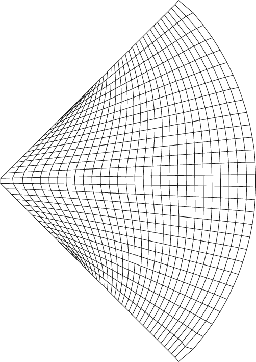
In Figure 31, the area concerned is that of an ellipse. In Figure 32, the domain is of a symmetrical diamond. This type of domain is interested in the wings of supersonic aircraft, where the airfoil should be pointed at the leading edge as the figure shows.

Figure 31.

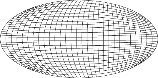
Quadrilateral mesh in an ellipse with N_x  = 30 and N_y  = 30.

Figure 32.

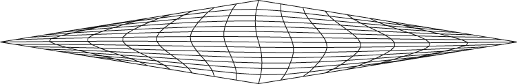
Quadrilateral mesh in a symmetrical diamond with N_x  = 15 and N_y  = 15.

In these figures, we chose N_x  = 30 and N_y  = 30. Then, the number of nodes equals 900 nodes, and therefore, the number of quadrilateral elements is equal to 841.

The difference between the presented meshes is only the boundary that varies. Meshes’ simple configuration can be found to build and the other as complex polygons and the airfoil.

In our application, we used several types of airfoils affecting all airlines. Part mesh generation is necessary to make the resolution of the Poisson equation.

The example shown in Figures 33 and 34 is the RAE 2822 airfoil with asymmetric camber. This area is of great interest to researchers interested in aerodynamics and elasticity. For example, if we can search and study the problem of torsion of helicopter blades, the propeller blades of the engine, the compressor blades, and other cases, it is necessary to generate this kind of mesh. Assume that we want to determine the area and geometric characteristics (position of the center of gravity, moments, and products of inertia) as a wing profile that will serve us for a study of strength and stiffness, we are still interested in this type of mesh. In Figure 35, we did not take an orthonormal mark in order to visualize the internal cells.

Figure 33.

Quadrilateral mesh in the RAE 2822 airfoil with N_x  = 10 and N_y  = 10.

Figure 34.

Quadrilateral mesh in the RAE 2822 airfoil with N_x  = 30 and N_y  = 30.

Figure 35.

Variation in the torsion parameters I_P , C, and τ_max /(2M_t ) versus the number of nodes of the discretization for the square.

Effect of discretization on the convergence

We consider the example of the square inscribed in a circle of radius R = 1.00 (see Figure 17). In this case, the length of each side is equal to $R\sqrt{2}$ —the choice of the square since we know the exact solution for the twist flow, as well as the distribution of torsional stress. In this case, and for R = 1.00, we have the following results. Then, I_P  = 0.666666, C = 0.555555, and τ_max /M_t  = 1.590990. The maximum stress occurs at the boundary on the middle points on each side of the square. This is the closest distance of the center of gravity. It is noted that the variable declaration is made in double precision. We consider the case N_x  = N_y since the dimensional x and y have the same length for the case of square.

Table 1 presents the results obtained on the polar moment of inertia, torsional constant, and the value of the maximum torque stress depending on the discretization. We clearly notice the convergence of these parameters to the exact solution.

Table 1.

Effect of discretization on the results for the square.

Nx  = Ny	IP	C	τmax/Mt
10	0.654340	0.550022	1.603855
20	0.664541	0.558885	1.673216
50	0.666674	0.561739	1.689697
80	0.666909	0.562084	1.693005
100	0.666964	0.562163	1.694256
120	0.666993	0.562206	1.694910
150	0.667017	0.562242	1.695659
180	0.667029	0.562261	1.696093
200	0.667035	0.562270	1.696345
250	0.667044	0.562283	1.696752
300	0.667048	0.562290	1.697030

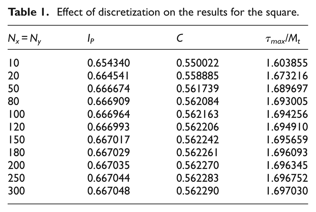
According to Table 2, the relative error obtained decreases as the number of nodes increases. So, for discretization N_x  = N_y  = 300 knots, it will be an error that stabilizes at ε_I  = 0.05%, ε_C  = 1.21%, and ε_τ  = 6.66% for I_P , C, and τ_max , respectively.

Table 2.

Errors obtained from the discretization of the square area.

Nx  = Ny	εI (%)	εC (%)	ετ (%)
10	1.848	0.995	0.808
20	0.318	0.599	5.168
50	0.001	1.113	6.204
80	0.036	1.175	6.412
100	0.044	1.189	6.490
120	0.049	1.197	6.531
150	0.052	1.203	6.578
180	0.054	1.207	6.606
200	0.055	1.208	6.621
250	0.056	1.210	6.647
300	0.057	1.212	6.665

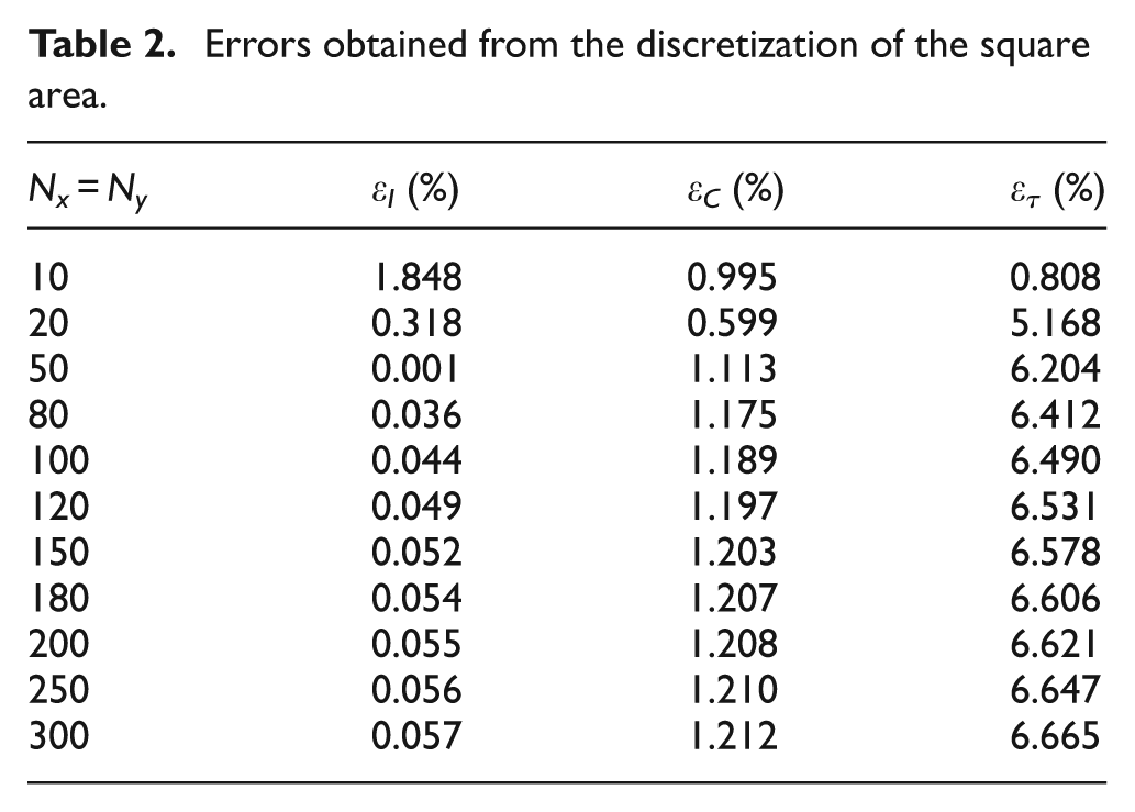
About the obtained error of 6.66% on the maximum stress, here the stress is obtained from the derivative of the primary solution which is the flow of twist, which is itself a first-order approximation. If we calculate the relative error on the flow of torsion, we will get an error ε = 0.02% for the discretization of N_x  = N_y  = 300 nodes. This error influences and will give us another error on the maximum stress. In addition, the finite element used affects the error obtained. Similarly, the error depends on the discretization, given the large number of mathematical operations performed. It gave us an error of 6.66%, which is an acceptable error.

Figure 35 shows the effect of the discretization on the convergence of the problem, especially the torsional constant, the polar moment of inertia, and the maximum stress of torsion for the square section. Note that if we increase the number of nodes NN of the discretization, we will clear the convergence of these parameters. In this case, we took N_x  = N_y since the dimension along the x-axis is the same as the dimension along the y-axis of the square section (see Figure 17).

The second example chosen is the geometry of an airfoil. The selected profile is the RAE 2822 with asymmetric camber. The definition of the geometry is presented by 65 points as shown in Table 3.^23,24 The points of Table 3 are used to determine the analytical function of the extrados and the intrados of using cubic spline interpolation. As the dimension along the vertical axis is about 10 times lower with respect to the longitudinal dimension, it takes N_x  = N_y /5. The exact solution in this case does not exist for the parameters shown in Table 3.

Table 3.

Defining points of the surface of the airfoil RAE 2822.

	x/Chord (%)	Extrados; En (%) of chord	Intrados; En (%) of chord
		y/Chord (%)	y/Chord (%)
01	0.0000	0.0000	0.0000
02	0.0602	0.3165	−0.3160
03	0.2408	0.6306	−0.6308
04	0.5412	0.9416	−0.9443
05	0.9607	1.2480	−1.2559
06	1.4984	1.5489	−1.5649
07	2.1530	1.8441	−1.8707
08	2.9228	2.1348	−2.1722
09	3.8060	2.4219	−2.4685
10	4.8005	2.7062	−2.7586
11	5.9039	2.9874	−3.0416
12	7.1136	3.2644	−3.3170
13	8.4265	3.5360	−3.5843
14	9.8396	3.8011	−3.8431
15	11.3495	4.0585	−4.0929
16	12.9524	4.3071	−4.3326
17	14.6447	4.5457	−4.5610
18	16.4221	4.7729	−4.7773
19	18.2803	4.9874	−4.9805
20	20.2150	5.1885	−5.1694
21	22.2215	5.3753	−5.3427
22	24.2949	5.5470	−5.4994
23	26.4302	5.7026	−5.6376
24	28.6222	5.8414	−5.7547
25	30.8658	5.9629	−5.8459
26	33.1555	6.0660	−5.9046
27	35.4858	6.1497	−5.9236
28	37.8510	6.2133	−5.8974
29	40.2455	6.2562	−5.8224
30	42.6635	6.2779	−5.6979
31	45.0991	6.2774	−5.5257
32	47.5466	6.2530	−5.3099
33	50.0000	6.2029	−5.0563
34	52.4534	6.1254	−4.7719
35	54.9009	6.0194	−4.4642
36	57.3365	5.8845	−4.1397
37	59.7545	5.7218	−3.8043
38	62.1490	5.5344	−3.4631
39	64.5142	5.3258	−3.1207
40	66.8445	5.0993	−2.7814
41	69.1342	4.8575	−2.4495
42	71.3778	4.6029	−2.1289
43	73.5698	4.3377	−1.8232
44	75.7051	4.0641	−1.5357
45	77.7785	3.7847	−1.2690
46	79.7850	3.5017	−1.0244
47	81.7197	3.2176	−0.8027
48	83.5779	2.9347	−0.6048
49	85.3553	2.6554	−0.4314
50	87.0476	2.3817	−0.2829
51	88.6505	2.1153	−0.1592
52	90.1604	1.8580	−0.0600
53	91.5735	1.6113	0.0157
54	92.8864	1.3769	0.0694
55	94.0961	1.1562	0.1033
56	95.1995	0.9508	0.1197
57	96.1940	0.7622	0.1212
58	97.0772	0.5915	0.1112
59	97.8470	0.4401	0.0935
60	98.5016	0.3092	0.0719
61	99.0393	0.2001	0.0497
62	99.4588	0.1137	0.0296
63	99.7592	0.0510	0.0137
64	99.9398	0.0128	0.0035
65	100.0000	0.0000	0.0000

According to Table 4, we can estimate from the discretization that I_P  = 0.00389, C = 0.25 × 10⁻³, and τ_max /M_t  = 452.

Table 4.

Effect of discretization on the results for the airfoil RAE 2822.

Nx	IP  × 100	C × 1000	τmax /Mt
20	0.370332	0.195192	421.340907
50	0.392467	0.240049	533.990253
80	0.392170	0.245799	557.266527
100	0.385273	0.247247	563.674954
150	0.388690	0.248807	569.357837
200	0.390404	0.249376	440.179398
250	0.387818	0.249719	443.746902
300	0.388899	0.249869	446.554339
350	0.389734	0.249924	448.722860
400	0.390395	0.250001	450.323953
420	0.388883	0.253347	450.745781
500	0.389447	0.250072	452.780371

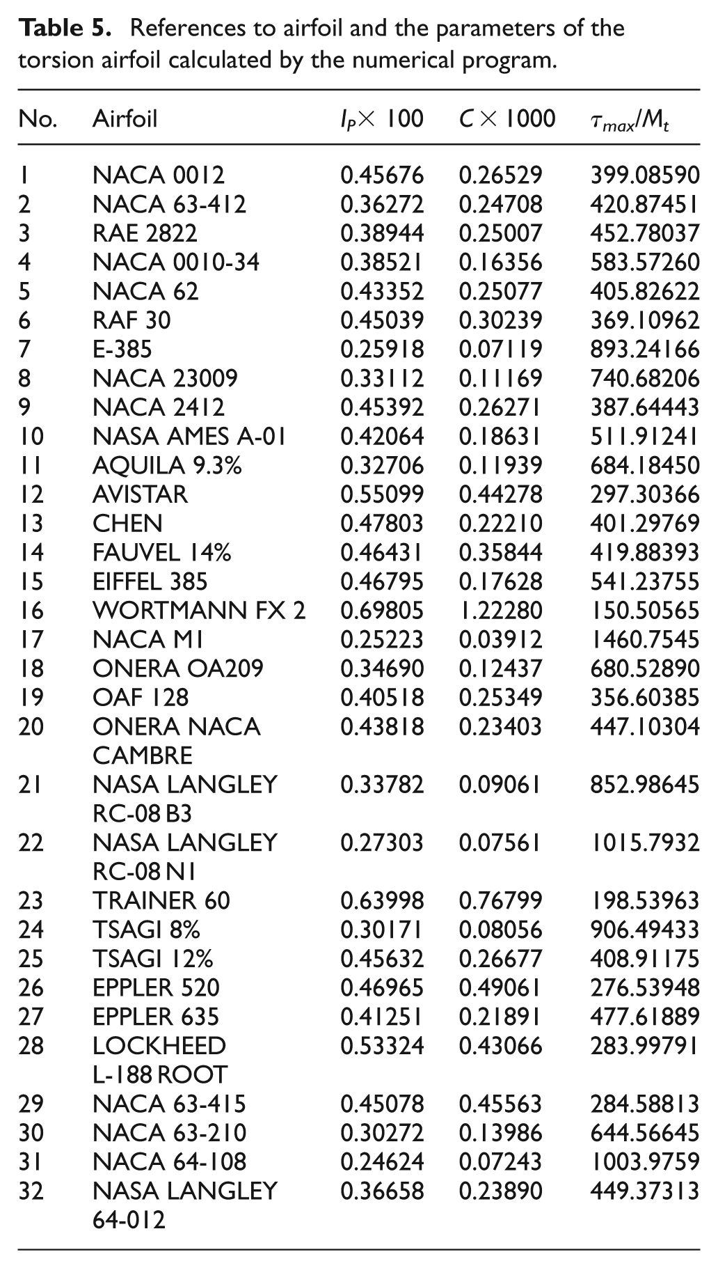
It was noted that the maximum torsional stress is applied on the boundary to the nearest center of gravity issue. Tables 5–7 present the results of our numerical calculation program on the torsional parameters for the wings and profiles for other interesting sections.

Table 5.

References to airfoil and the parameters of the torsion airfoil calculated by the numerical program.

No.	Airfoil	IP × 100	C × 1000	τmax /Mt
1	NACA 0012	0.45676	0.26529	399.08590
2	NACA 63-412	0.36272	0.24708	420.87451
3	RAE 2822	0.38944	0.25007	452.78037
4	NACA 0010-34	0.38521	0.16356	583.57260
5	NACA 62	0.43352	0.25077	405.82622
6	RAF 30	0.45039	0.30239	369.10962
7	E-385	0.25918	0.07119	893.24166
8	NACA 23009	0.33112	0.11169	740.68206
9	NACA 2412	0.45392	0.26271	387.64443
10	NASA AMES A-01	0.42064	0.18631	511.91241
11	AQUILA 9.3%	0.32706	0.11939	684.18450
12	AVISTAR	0.55099	0.44278	297.30366
13	CHEN	0.47803	0.22210	401.29769
14	FAUVEL 14%	0.46431	0.35844	419.88393
15	EIFFEL 385	0.46795	0.17628	541.23755
16	WORTMANN FX 2	0.69805	1.22280	150.50565
17	NACA M1	0.25223	0.03912	1460.7545
18	ONERA OA209	0.34690	0.12437	680.52890
19	OAF 128	0.40518	0.25349	356.60385
20	ONERA NACA CAMBRE	0.43818	0.23403	447.10304
21	NASA LANGLEY RC-08 B3	0.33782	0.09061	852.98645
22	NASA LANGLEY RC-08 N1	0.27303	0.07561	1015.7932
23	TRAINER 60	0.63998	0.76799	198.53963
24	TSAGI 8%	0.30171	0.08056	906.49433
25	TSAGI 12%	0.45632	0.26677	408.91175
26	EPPLER 520	0.46965	0.49061	276.53948
27	EPPLER 635	0.41251	0.21891	477.61889
28	LOCKHEED L-188 ROOT	0.53324	0.43066	283.99791
29	NACA 63-415	0.45078	0.45563	284.58813
30	NACA 63-210	0.30272	0.13986	644.56645
31	NACA 64-108	0.24624	0.07243	1003.9759
32	NASA LANGLEY 64-012	0.36658	0.23890	449.37313

Table 6.

Parameters of the twist for various sections calculated by the numerical program.

No.	Section	IP	C	τmax /Mt
1	Half-circle	0.497787	0.295882	2.824595
2	Quarter circle	0.109622	0.082265	6.828792
3	Diamond	0.057088	0.005809	47.217214
4	Astroid	0.257599	0.159554	4.859267
	Ellipse	0.490792	0.314019	2.520921

Table 7.

Parameters of the twisting for regular polygons calculated by the numerical program.

No.	Regular polygon	IP	C	τmax /Mt
1	3 sides	0.321788	0.194179	3.858309
2	4 sides	0.666985	0.562223	1.597483
3	5 sides	0.912464	0.843477	1.220653
4	6 sides	1.079139	1.033943	1.008196
5	7 sides	1.196632	1.163550	0.920556
6	8 sides	1.276903	1.252984	0.856709
7	9 sides	1.333891	1.316137	0.805976
8	10 sides	1.376275	1.362921	0.777727
9	11 sides	1.408764	1.398027	0.760770
10	12 sides	1.432861	1.424582	0.743825
11	13 sides	1.454615	1.446645	0.726902
12	14 sides	1.469686	1.463530	0.716779
13	Circle	1.570537	1.570212	0.636754

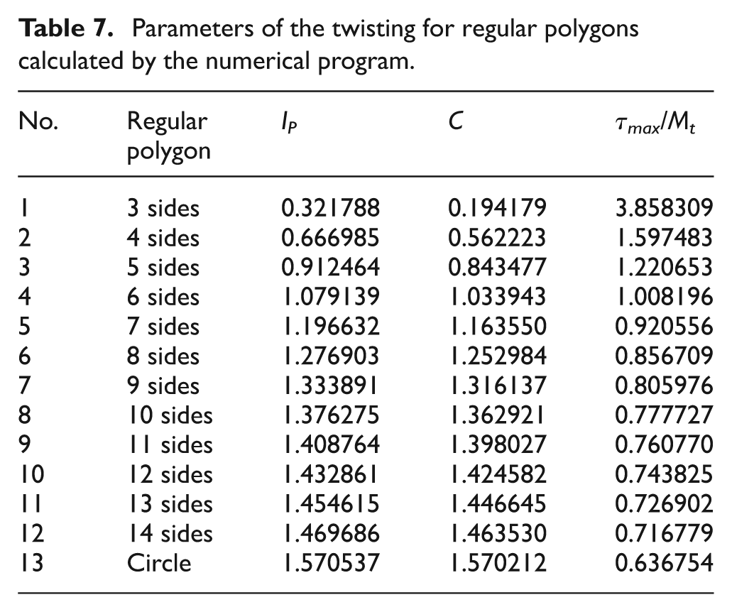
From Tables 5–7, we note that the torsional constant C is different to polar moment of inertia, and it is equal only to the circular section. This result demonstrates that the formulas of torsion for circular section beings cannot be applied to determine the angle and torsional stress for non-circular sections. For information, the strength of the materials use the formulas of circular section to solve the problems of non-circular cross sections due to lack of formulas for non-circular sections.

The selected data for an ellipse are that the dimension along the horizontal axis is equal to a = 1.00 and the dimension in the vertical axis is b = 0.50.

The exact formula for polar moment of inertia for regular polygons of n (n ≥ 3) sides inscribed in a circle of radius R is given by^1,4

$$I_P=\frac{{\mathrm{nR}}^4}{12}\sin \frac{2\pi }{n}[2+\cos \frac{2\pi }{n}]$$

(82)

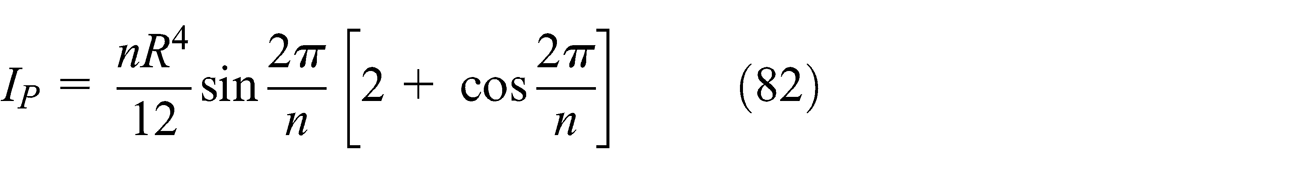
Similarly, the value of the torsion constant and the maximum torsional stress for some regular polygons appear in Table 8.^1,4

Table 8.

Exacts of torsional parameters for regular polygons. ¹

No.	Regular polygon	IP (exact)	C (exact)	τmax /Mt (exact)
1	3 sides	0.32475952	0.19485571	3.84900179
2	4 sides	0.66666666	0.55555555	1.59099025
3	6 sides	1.08253175	1.03831376	1.02009999
4	8 sides	1.27614237	1.25510511	0.85671294
5	Circle	1.57079632	1.57079632	0.63661977

The errors obtained for these parameters are presented in Table 9. Note that the error is very small for a discretization N_x  = N_y  = 200. If we increase the number of nodes in the discretization, we will see an error lower than that presented in Table 9.

Table 9.

Errors obtained on torsional parameters for some regular polygons.

No.	Regular polygon	ε (%) of IP	ε (%) of C	ε (%) of τmax /Mt
1	3 sides	0.752	0.213	0.171
2	4 sides	0.023	0.802	0.302
3	6 sides	0.281	0.357	0.925
4	8 sides	0.042	0.905	0.00046
5	Circle	0.012	0.027	0.019

For the circular section, we obtained an error approximately 0.01% for all parameters for discretization N_x  = N_y  = 200. Note that we did not find the exact solution for sections of airfoils in the literature.

Conclusion

This work allows us to make the determination of the torsional stress in any non-circular sections by the finite element method using a four-node quadrilateral element and make applications for airfoil used in aeronautics. The following points can be drawn from this work:

1. The problem can be seen as the mathematical resolution of the Poisson equation in a 2D simply connected domain by the finite element method with Dirichlet boundary conditions.

2. Various fields have been presented in this work involving many disciplines implicitly.

3. Section must be set in the center mark of the section.

4. All airfoils considered are presented in the tabulated values. The cubic spline interpolation is used in this case to obtain an analytic function of the upper and lower surfaces.

5. Condensation nodes to the leading edge of the airfoil are used to refine the points to the edge having the large curvature in this region.

6. An optional filter node is used to reposition the internal nodes of the mesh to solve the problem of cell sizes obtained.

7. Comparing the results to determine the accuracy of the developed program was made for the square domain, the exact solution exists.

8. The maximum stress is shown on the boundary closest to the center of gravity points.

9. The torsional constant is equal to the value of polar moment of inertia for circular section, and it is different for the non-circular case.

10. We cannot apply the torsion formulas of circular section to determine the angle and torsional stress for non-circular sections. This is the case for the strength of the materials’ discipline.

11. Solving the system of equations obtained is done with the technique of matrix bands when storing the upper part of the band matrix is considered in a vector because the stiffness matrix is symmetric and wide.

12. The algorithm for solving the used system of equations is Khaletski designed specifically for the direct solution of systems of equations. Transfer boxes between the matrix and the corresponding vector are done by the diagonal-by-diagonal manner.

13. The numerical program developed can solve a very high-order equation system, which can reach millions or even higher.

14. Problems with the Neumann boundary conditions and Cauchy are left as future work.

15. As future work, we can do the calculation extension for doubly or even multi-connected domain.